TensorFlow和Keras,在之前我们都用过了。 现在,我们专门用两章分别讨论TensorFlow和Keras,是归纳总结,也是查漏补缺。
TensorFlow是一个面向深度学习算法的科学计算库,内部数据保存在张量(Tensor)对象上,所有的运算操作(Operation,简称 OP)也都是基于张量对象进行的。
数据类型
首先,我们来讨论一下TensorFlow中的几个基本数据类型:
数值类型
布尔类型
字符串类型
数值类型
我想什么是数值型数据,这个大家都已经知道了,顾名思义即可。
标量
向量
矩阵
张量
标量
标量(Scalar)。单个的实数,如1.2,3.4等,维度(Dimension)数为0,形状(Shape)为()。
1 2 print(tf.constant(1 )) print(tf.constant(1.0 ))
运行结果:
1
2
tf.Tensor(1, shape=(), dtype=int32) tf.Tensor(1.0, shape=(), dtype=float32)
向量
向量(Vector)。n n n [1.2],[1.2,3.4],维度数为1,长度不定,形状为(n,)。
1 2 3 print(tf.constant([1 ,2 ,3 ,4 ])) print(tf.constant([1.2 ,3.4 ])) print(tf.constant([1 ,2 ,3.4 ]))
运行结果:
1
2
3
tf.Tensor([1 2 3 4], shape=(4,), dtype=int32) tf.Tensor([1.2 3.4], shape=(2,), dtype=float32) tf.Tensor([1. 2. 3.4], shape=(3,), dtype=float32)
矩阵
矩阵(Matrix)。n n n m m m [[1,2],[3,4]],也可以写成
[ 1 2 3 4 ] \left[
\begin{matrix}
1 & 2 \\
3 & 4
\end{matrix}
\right]
[ 1 3 2 4 ]
维度数为2,每个维度上的长度不定,形状为(n,m)。
1 2 3 print(tf.constant([[1 ,2 ],[3 ,4 ]])) print(tf.constant([[1 ,2 ],[3.0 ,4.0 ]])) print(tf.constant([[1.0 ,2.0 ],[3.0 ,4.0 ]]))
运行结果:
1
2
3
4
5
6
7
8
9
tf.Tensor( [[1 2] [3 4]], shape=(2, 2), dtype=int32) tf.Tensor( [[1. 2.] [3. 4.]], shape=(2, 2), dtype=float32) tf.Tensor( [[1. 2.] [3. 4.]], shape=(2, 2), dtype=float32)
张量
张量(Tensor)。所有维度数dim>2的数组统称为张量,张量的每个维度也作轴(Axis)。
例如,在图片数据中,通常约定,形状为(2,32,32,3)的4维张量,其四个维度/轴代表的含义依次是图片数量、图片高度、图片宽度、图片通道数。
2代表了2张图片第一个32代表高
第二个32代表宽
3代表了RGB共3个通道
示例代码:
1
2
tensor = tf.constant([[[1 ,2 ],[3 ,4 ]],[[5 ,6 ],[7 ,8 ]]]) print(tensor)
运行结果:
1
2
3
4
5
6
tf.Tensor( [[[1 2] [3 4]] [[5 6] [7 8]]], shape=(2, 2, 2), dtype=int32)
小结
数值类型
维度数
形状
例子
标量(Scalar)
0
()1
向量(Vector
1
(n,)[1,2]
矩阵(Matrix)
2
(n,m)[[1,2],[3,4]]
张量(Tensor)
≥ 2 \geq 2 ≥ 2 (n,m,i···)[[1,2],[3,4]],[[5,6],[7,8]]]
特别注意: 在TensorFlow中,为了表达方便,一般把标量、向量、矩阵统称为张量,不作区分,需要根据维度数或形状自行判断。
布尔类型
布尔类型的张量只需要传入Python语言的布尔类型数据,转换成TensorFlow的布尔类型即可。
1
2
3
4
scalar = tf.constant(True ) print(scalar) vector = tf.constant([True ,False ]) print(vector)
运行结果:
1
2
tf.Tensor(True, shape=(), dtype=bool) tf.Tensor([ True False], shape=(2,), dtype=bool)
示例代码:
1
2
3
4
5
6
7
tf_true = tf.constant(True ) print(type(tf_true)) print(type(True )) print(tf_true is True ) print(tf_true == True ) print(tf_true == tf_true) print(tf_true.numpy() == True )
运行结果:
1
2
3
4
5
6
<class 'tensorflow.python.framework.ops.EagerTensor'> <class 'bool'> False tf.Tensor(True, shape=(), dtype=bool) tf.Tensor(True, shape=(), dtype=bool) True
注意:
TensorFlow中的的布尔类型和Python语言的布尔类型的比较,返回的是TensorFlow中的的布尔类型。
TensorFlow中的的布尔类型的"numpy()"和Python语言的布尔类型的比较,返回的是Python语言的布尔类型。
字符串类型
除了数值类型和布尔类型外,TensorFlow还支持字符串(String)类型的数据,而且还提供了常见的字符串类型的工具函数,如:lower()、upper()、join()、length()、split()等。
1
2
3
4
5
6
7
string = tf.constant('Deep Learning' ) print(string) print(tf.strings.lower(string)) print(tf.strings.upper(string)) print(tf.strings.join([string,string])) print(tf.strings.length(string)) print(tf.strings.split(string,' ' ))
运行结果:
1
2
3
4
5
6
tf.Tensor(b'Deep Learning', shape=(), dtype=string) tf.Tensor(b'deep learning', shape=(), dtype=string) tf.Tensor(b'DEEP LEARNING', shape=(), dtype=string) tf.Tensor(b'Deep LearningDeep Learning', shape=(), dtype=string) tf.Tensor(13, shape=(), dtype=int32) tf.Tensor([b'Deep' b'Learning'], shape=(2,), dtype=string)
数值精度
深度学习算法主要还是以数值类型张量的运算为主,所以我们主要讨论数值类型,而数值类型又有多种,代表着不同的精度。
常见精度
常用的精度有:tf.int16、tf.int32、tf.int64、tf.float16、tf.float32、tf.float64等,其中tf.float64即为tf.double。
默认数据类型:
不带小数点的数会被默认为tf.int32。
带小数点的会被默认为tf.float32。
这个我们在上一小节讨论数值类型的时候,通过示例代码和运行结果,已经感受过了。
对于大部分深度学习算法,一般使用tf.int32和tf.float32也就够了。部分对精度要求较高的算法,可以选择使用tf.int64和tf.float64。
读取精度
通过张量的dtype属性读取精度。
1
2
float32 = tf.constant([1.2,1]) print(float32.dtype)
运行结果:
类型转换
在TensorFlow中,只要dtype不同,就无法进行运算。
1 2 3 4 5 6 print(1.0 +1 ) float32 = tf.constant(1.0 ) int32 = tf.constant(1 ) print(float32.dtype) print(int32.dtype) print(tf.constant(1.0 ) + tf.constant(1 ))
运行结果:
1
2
3
4
5
6
7
2.0 <dtype: 'float32'> <dtype: 'int32'> 【部分运行结果略】 InvalidArgumentError: cannot compute AddV2 as input #1(zero-based) was expected to be a float tensor but is a int32 tensor [Op:AddV2]
如果一定要进行运行,则需要进行类型转换。
示例代码:
1
2
3
4
float32 = tf.constant(1.0 ) int32 = tf.constant(1 ) int32 = tf.cast(x=int32,dtype=tf.float32) print(float32 + int32)
运行结果:
1 tf.Tensor(2.0, shape=(), dtype=float32)
特别注意:将高精度的张量转换为低精度的张量时,会丢失精度。
1
2
float_1_2 = tf.constant(1.2 ) print(tf.cast(x=float_1_2,dtype=tf.int32))
运行结果:
1 tf.Tensor(1, shape=(), dtype=int32)
布尔类型与整型也可以进行相互转换,同样是False是0,True是1,非0数字都视为True。
1 2 3 print(tf.cast(tf.constant(True ),dtype=tf.int32)) print(tf.cast(tf.constant(False ),dtype=tf.int32)) print(tf.cast(tf.constant(2 ),dtype=tf.bool))
运行结果:
1
2
3
tf.Tensor(1, shape=(), dtype=int32) tf.Tensor(0, shape=(), dtype=int32) tf.Tensor(True, shape=(), dtype=bool)
指定精度
我们也可以在创建张量的时候,指定精度。
1 print(tf.constant(1 ,dtype=tf.float32))
运行结果:
1 tf.Tensor(1.0, shape=(), dtype=float32)
张量的创建
在TensorFlow中,可以通过多种方式创建张量,如从Python列表对象创建,从Numpy数组创建,或者创建某种已知分布的张量等。
从数组、列表对象创建
tf.constant()和tf.convert_to_tensor()都能够自动的把Python列表或者Numpy数组数据类型转化为Tensor类型。
1 2 3 4 5 print(tf.constant([1 ,2 ])) print(tf.constant(np.array([1 ,2 ]))) print(tf.convert_to_tensor([1 ,2 ])) print(tf.convert_to_tensor(np.array([1 ,2 ])))
运行结果:
1
2
3
4
tf.Tensor([1 2], shape=(2,), dtype=int32) tf.Tensor([1 2], shape=(2,), dtype=int32) tf.Tensor([1 2], shape=(2,), dtype=int32) tf.Tensor([1 2], shape=(2,), dtype=int32)
创建全 0 或全 1 张量
通过tf.zeros()和tf.ones()即可创建任意形状,且内容全0或全1的张量。
1
2
print(tf.zeros([3,2])) print(tf.ones([3,2]))
运行结果:
1
2
3
4
5
6
7
8
tf.Tensor( [[0. 0.] [0. 0.] [0. 0.]], shape=(3, 2), dtype=float32) tf.Tensor( [[1. 1.] [1. 1.] [1. 1.]], shape=(3, 2), dtype=float32)
通过tf.zeros_like(),tf.ones_like()可以方便地新建与某个张量shape一致,且内容为全0或全1的张量。
1
2
3
4
5
6
7
a = tf.constant([[1 ,2 ],[3 ,4 ]]) print(tf.zeros(a.shape)) print(tf.zeros_like(a)) print(tf.ones(a.shape)) print(tf.ones_like(a))
运行结果:
1
2
3
4
5
6
7
8
9
10
11
12
tf.Tensor( [[0. 0.] [0. 0.]], shape=(2, 2), dtype=float32) tf.Tensor( [[0 0] [0 0]], shape=(2, 2), dtype=int32) tf.Tensor( [[1. 1.] [1. 1.]], shape=(2, 2), dtype=float32) tf.Tensor( [[1 1] [1 1]], shape=(2, 2), dtype=int32)
创建自定义数值张量
通过tf.fill(shape, value)可以创建全为自定义数值value的张量,形状由shape参数指定。
1 2 3 4 5 6 7 print(tf.fill([],-1 )) print(tf.fill([1 ],-1 )) print(tf.fill([2 ,2 ],-1 )) print(tf.fill([2 ,2 ,2 ],-1 )) a = tf.constant([[1 ,2 ],[3 ,4 ]]) print(tf.fill(a.shape,-1 ))
运行结果:
1
2
3
4
5
6
7
8
9
10
11
12
13
14
tf.Tensor(-1, shape=(), dtype=int32) tf.Tensor([-1], shape=(1,), dtype=int32) tf.Tensor( [[-1 -1] [-1 -1]], shape=(2, 2), dtype=int32) tf.Tensor( [[[-1 -1] [-1 -1]] [[-1 -1] [-1 -1]]], shape=(2, 2, 2), dtype=int32) tf.Tensor( [[-1 -1] [-1 -1]], shape=(2, 2), dtype=int32)
创建已知分布的张量
通过tf.random.normal(shape, mean=0.0, stddev=1.0)可以创建形状为shape,指定均值,指定标准差的的正态分布( m e a n , s t d d e v 2 ) (mean,{stddev}^2) ( m e a n , s t d d e v 2 )
1 2 print(tf.random.normal([2 ,2 ])) print(tf.random.normal([2 ,2 ],mean=100 ,stddev=1 ))
运行结果:
1
2
3
4
5
6
tf.Tensor( [[ 0.30633727 0.68629885] [ 1.7981079 -0.23062594]], shape=(2, 2), dtype=float32) tf.Tensor( [[ 99.23877 99.06489 ] [100.07093 98.131874]], shape=(2, 2), dtype=float32)
通过tf.random.uniform(shape, minval=0, maxval=None, dtype=tf.float32)可以创建采样自[minval, maxval)区间的均匀分布的张量。
1 2 print(tf.random.uniform([2 ,2 ], minval=0 , maxval=None )) print(tf.random.uniform([2 ,2 ], minval=0 , maxval=100 ))
运行结果:
1
2
3
4
5
6
tf.Tensor( [[0.14329934 0.9274646 ] [0.19031143 0.7906921 ]], shape=(2, 2), dtype=float32) tf.Tensor( [[18.60162 27.118896] [99.79489 85.88089 ]], shape=(2, 2), dtype=float32)
如果需要均匀采样整形类型的数据,必须指定采样区间的最大值maxval参数,同时指定数据类型为tf.int*型
1
2
print(tf.random.uniform([2,2], minval=0, maxval=100,dtype=tf.int32)) print(tf.random.uniform([2,2], minval=0, maxval=None,dtype=tf.int32))
运行结果:
1
2
3
4
5
6
7
tf.Tensor( [[77 99] [63 98]], shape=(2, 2), dtype=int32) 【部分运行结果略】 ValueError: Must specify maxval for integer dtype tf.int32
创建序列
通过tf.range(start,limit, delta)可以创建[start, limit)之间,步长为delta的整型序列,不包含limit本身。
1 print(tf.range(start=1 , limit=10 , delta=1 ))
运行结果:
1 tf.Tensor([1 2 3 4 5 6 7 8 9], shape=(9,), dtype=int32)
变量,一种特殊的张量
我们注意到刚刚我们创建张量,有一个方法是tf.constant()。
constant:adj. 不变的;恒定的;经常的。n. 常数;恒量。
那么,既然有不变的,似乎就应该有变的:tf.Variable()。
TensorFlow中一种专门用来记录梯度的数据类型,tf.Variable,变量。tf.Variable类型在普通的张量类型基础上添加了name,trainable等属性来支持计算图的构建。
通过tf.Variable()函数可以将普通张量转换为变量。
1
2
3
4
5
6
7
8
9
10
11
12
13
14
cons = tf.constant([1 , 2 ]) print(cons) try : print(cons.name,cons.trainable) except Exception as e: print(e) var = tf.Variable([1 ,2 ]) print(var) print(var.name,var.trainable) cons2var = tf.Variable(cons) print(cons2var) print(cons2var.name,cons2var.trainable)
运行结果:
1
2
3
4
5
6
tf.Tensor([1 2], shape=(2,), dtype=int32) Tensor.name is meaningless when eager execution is enabled. <tf.Variable 'Variable:0' shape=(2,) dtype=int32, numpy=array([1, 2])> Variable:0 True <tf.Variable 'Variable:0' shape=(2,) dtype=int32, numpy=array([1, 2])> Variable:0 True
索引和切片
通过索引与切片操作可以提取张量的部分数据。
索引
在TensorFlow中,支持基本的[i][j]···标准索引方式,也支持通过逗号分隔索引号的[i,j···]索引方式。4张32*32的3通道彩色图片,形状为[4,32,32,3]。
取第1张图片的数据
1
2
x = tf.random.normal([4 ,32 ,32 ,3 ]) print(x[0 ])
运行结果:
1
2
3
4
5
6
7
8
9
10
tf.Tensor( [[[-1.1012203 1.5457517 0.383644 ] [-0.87965786 -1.2246722 -0.9811211 ] [ 0.08780783 -0.20326038 -0.5581562 ] 【部分运行结果略】 [ 0.05611933 1.1054882 1.0421329 ] [-0.75182426 0.4644055 0.39869747] [ 2.2079358 0.712941 -1.2138437 ]]], shape=(32, 32, 3), dtype=float32)
取第1张图片的第2行
1
2
3
x = tf.random.normal([4 ,32 ,32 ,3 ]) print(x[0 ][1 ]) print(x[0 ,1 ])
运行结果:
1
2
3
4
5
6
7
8
9
10
11
12
13
14
15
16
17
18
19
20
tf.Tensor( [[-0.2077277 -1.0625398 1.6242949 ] [ 0.9868854 1.0166248 -0.7334497 ] [-0.4377686 0.80627435 0.7412633 ] 【部分运行结果略】 [-0.33113936 0.09343005 -0.79938453] [ 1.8220028 1.923281 0.51009125] [-1.4206531 1.4717104 -1.4910527 ]], shape=(32, 3), dtype=float32) tf.Tensor( [[-0.2077277 -1.0625398 1.6242949 ] [ 0.9868854 1.0166248 -0.7334497 ] [-0.4377686 0.80627435 0.7412633 ] 【部分运行结果略】 [-0.33113936 0.09343005 -0.79938453] [ 1.8220028 1.923281 0.51009125] [-1.4206531 1.4717104 -1.4910527 ]], shape=(32, 3), dtype=float32)
取第1张图片,第2行,第3列
1
2
3
x = tf.random.normal([4 ,32 ,32 ,3 ]) print(x[0 ][1 ][2 ]) print(x[0 ,1 ,2 ])
运行结果:
1
2
tf.Tensor([-0.4377686 0.80627435 0.7412633 ], shape=(3,), dtype=float32) tf.Tensor([-0.4377686 0.80627435 0.7412633 ], shape=(3,), dtype=float32)
取第1张图片,第2行,第3列,第1个通道。
1
2
3
x = tf.random.normal([4 ,32 ,32 ,3 ]) print(x[0 ][1 ][2 ][0 ]) print(x[0 ,1 ,2 ,0 ])
运行结果:
1
2
tf.Tensor(-0.4377686, shape=(), dtype=float32) tf.Tensor(-0.4377686, shape=(), dtype=float32)
即,索引从最大的层级开始找。(就像我们在图书馆找书,先确定楼层。)
切片
通过start:end:step切片方式可以方便地提取一段数据,其中start为开始读取位置的索引,end为结束读取位置的索引(不包含end位),step为采样步长。start:end:step切片方式有很多简写方式:
如果start不填的话,说明从0开始。
如果end不填的话,说明到最后。
如果step不填的话,说明步长是1。
特别的,我们不但可以不写step,还可以不写step左边的:
切片用:分隔,索引用,分隔。这几种排列组合又有多种情况。
从第2张图片开始,到第4张(不含),步长为1
1
2
3
x = tf.random.normal([4 ,32 ,32 ,3 ]) print(x[1 :3 ]) print(x[1 :3 :1 ])
运行结果:
1
2
3
4
5
6
7
8
9
10
11
12
13
14
15
16
17
18
19
20
tf.Tensor( [[[[ 0.3554342 0.10115115 -0.16103993] [ 0.01779328 0.46773523 -0.21666302] [ 1.124249 -0.54006565 1.3055763 ] 【部分运行结果略】 [-2.051547 -1.8475965 -1.8669469 ] [-0.18166229 0.03936828 0.6199849 ] [ 0.5860354 2.001519 -1.1584325 ]]]], shape=(2, 32, 32, 3), dtype=float32) tf.Tensor( [[[[ 0.3554342 0.10115115 -0.16103993] [ 0.01779328 0.46773523 -0.21666302] [ 1.124249 -0.54006565 1.3055763 ] 【部分运行结果略】 [-2.051547 -1.8475965 -1.8669469 ] [-0.18166229 0.03936828 0.6199849 ] [ 0.5860354 2.001519 -1.1584325 ]]]], shape=(2, 32, 32, 3), dtype=float32)
读取第1张图片
1
2
3
x = tf.random.normal([4 ,32 ,32 ,3 ]) print(x[0 ]) print(x[0 ,0 :,0 ::,::])
运行结果:
1
2
3
4
5
6
7
8
9
10
11
12
13
14
15
16
17
18
19
20
tf.Tensor( [[[-1.1012203 1.5457517 0.383644 ] [-0.87965786 -1.2246722 -0.9811211 ] [ 0.08780783 -0.20326038 -0.5581562 ] 【部分运行结果略】 [ 0.05611933 1.1054882 1.0421329 ] [-0.75182426 0.4644055 0.39869747] [ 2.2079358 0.712941 -1.2138437 ]]], shape=(32, 32, 3), dtype=float32) tf.Tensor( [[[-1.1012203 1.5457517 0.383644 ] [-0.87965786 -1.2246722 -0.9811211 ] [ 0.08780783 -0.20326038 -0.5581562 ] 【部分运行结果略】 [ 0.05611933 1.1054882 1.0421329 ] [-0.75182426 0.4644055 0.39869747] [ 2.2079358 0.712941 -1.2138437 ]]], shape=(32, 32, 3), dtype=float32)
特别的,step可以为负数,表示倒序,此时要求e n d ≤ s t a r t end \leq start e n d ≤ s t a r t
1
2
3
4
5
x = tf.range(10) print(x) print(x[::-1]) print(x[10::-1]) print(x[::-2])
运行结果:
1
2
3
4
tf.Tensor([0 1 2 3 4 5 6 7 8 9], shape=(10,), dtype=int32) tf.Tensor([9 8 7 6 5 4 3 2 1 0], shape=(10,), dtype=int32) tf.Tensor([9 8 7 6 5 4 3 2 1 0], shape=(10,), dtype=int32) tf.Tensor([9 7 5 3 1], shape=(5,), dtype=int32)
合并和分割
合并
合并的方法有两种:
拼接
堆叠
拼接
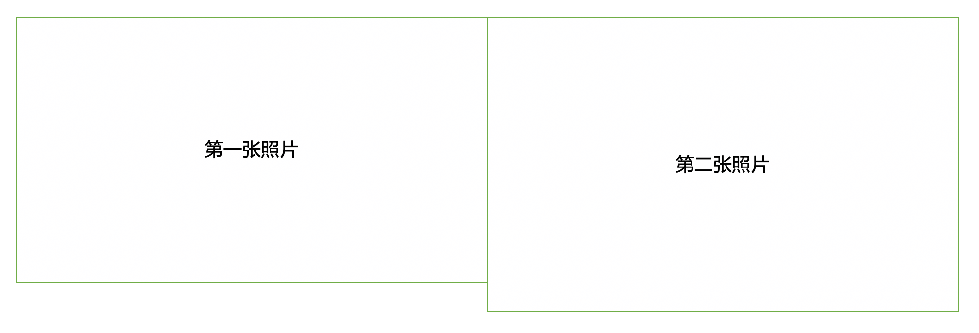
例如,现在我们有两张相片[h,w,c]:
第一张照片是[9,16,3],表示高是9,宽是16,3通道的彩色照片。
第二张照片是[10,16,3],表示高是10,宽是16,3通道的彩色照片。
现在,我们在高的维度,把两张照片拼接一张。即新照片高是19,宽是16,3通道的彩色照片。
1 2 3 4 5 6 tf.random.set_seed(1 ) a = tf.random.normal([9 ,16 ,3 ]) b = tf.random.uniform([10 ,16 ,3 ]) print(a.shape) print(b.shape) print(tf.concat([a,b],axis=0 ).shape)
运行结果:
1
2
3
(9, 16, 3) (10, 16, 3) (19, 16, 3)
那么,我们可以从宽的维度,把两张照片拼接成一张吗?当然不可以,就像这样:
1 2 3 4 5 6 tf.random.set_seed(1 ) a = tf.random.normal([9 ,16 ,3 ]) b = tf.random.uniform([10 ,16 ,3 ]) print(a.shape) print(b.shape) print(tf.concat([a,b],axis=1 ).shape)
运行结果:
1
2
3
4
5
6
(9, 16, 3) (10, 16, 3) 【部分运行结果略】 InvalidArgumentError: ConcatOp : Dimensions of inputs should match: shape[0] = [9,16,3] vs. shape[1] = [10,16,3] [Op:ConcatV2] name: concat
那么,我们可以把高和宽都一样的3通道彩色照片和1通道的黑白照片在高或宽的维度拼接一张吗?当然也不可以。我们可以理解通道数是厚度,两张厚度不一样的照片自然是没法拼接的。但是我们可以把两张拼接成一张4通道的照片啊。
1 2 3 4 5 6 7 8 9 10 11 12 13 tf.random.set_seed(1 ) a = tf.random.normal([9 ,16 ,3 ]) b = tf.random.uniform([9 ,16 ,1 ]) print(a.shape) print(b.shape) try : print(tf.concat([a,b],axis=0 ).shape) except Exception as e: print(e) try : print(tf.concat([a,b],axis=2 ).shape) except Exception as e: print(e)
运行结果:
1
2
3
4
(9, 16, 3) (9, 16, 1) ConcatOp : Dimensions of inputs should match: shape[0] = [9,16,3] vs. shape[1] = [9,16,1] [Op:ConcatV2] name: concat (9, 16, 4)
实际上的确存在4通道的照片,GIF格式的动态图。例如,GIf动态图:
拼接合并操作可以在任意的维度上进行,唯一的约束是非合并维度的长度必须一致。
堆叠
现在,我们要把两张照片堆叠成一组照片。这个要求就更高了,要求两张照片高度一样、宽度一样,连通道数都要一样。
1 2 3 4 5 6 tf.random.set_seed(1 ) a = tf.random.normal([9 ,16 ,3 ]) b = tf.random.uniform([9 ,16 ,3 ]) print(a.shape) print(b.shape) print(tf.stack([a,b],axis=0 ).shape)
运行结果:
1
2
3
(9, 16, 3) (9, 16, 3) (2, 9, 16, 3)
通常我们约定,在4个维度数表示照片的时候,第一个维度数是照片的数量。即[b,h,w,c],但我们也可以不遵守这个约定。
1 2 3 4 5 6 tf.random.set_seed(1 ) a = tf.random.normal([9 ,16 ,3 ]) b = tf.random.uniform([9 ,16 ,3 ]) print(a.shape) print(b.shape) print(tf.stack([a,b],axis=1 ).shape)
运行结果:
1
2
3
(9, 16, 3) (9, 16, 3) (9, 2, 16, 3)
分割
tf.split(x, num_or_size_splits, axis)可以完成张量的分割操作,参数意义如下:
x:待分割张量
num_or_size_splits:切割方案。
当 num_or_size_splits 为单个数值时,如 10,表示等长切割为 10 份;
当 num_or_size_splits 为 List 时,List 的每个元素表示每份的长度,如[2,4,2,2]表示切割为 4 份,每份的长度依次是 2、4、2、2。
axis 参数:指定分割的维度索引号。
比如,刚刚的那张照片。
1
2
3
4
5
x = tf.random.normal([9 ,16 ,3 ]) print(x.shape) splits = tf.split(value=x,num_or_size_splits=2 ,axis=1 ) print(splits[0 ].shape) print(splits[1 ].shape)
运行结果:
1
2
3
(9, 16, 3) (9, 8, 3) (9, 8, 3)
填充和复制
填充
刚刚我们讨论了,这样的两张照片是无法拼接的。
填充操作可以通过tf.pad(x, paddings)函数实现,参数paddings是包含了多个[Left Padding,Right Padding]的嵌套方案List,如[[0,0],[2,1],[1,2]]表示第一个维度不填充,第二个维度起始处填充两个单元,结束处填充一个单元,第三个维度左边填充一个单元,右边填充两个单元。
示例代码:
1
2
3
4
5
6
7
8
9
a = tf.constant([0 ,1 ,2 ]) print(a) try : print(tf.pad(a,[0 ,2 ])) except Exception as e: print(e) print(tf.pad(a,[[0 ,2 ]]))
运行结果:
1
2
3
tf.Tensor([0 1 2], shape=(3,), dtype=int32) paddings must be a matrix with 2 columns: [2] [Op:Pad] tf.Tensor([0 1 2 0 0], shape=(5,), dtype=int32)
特别注意:是[[0,2]],不是[0,2]
那么,对于我们刚刚讨论的那两张照片呢?
1
2
3
4
5
6
7
8
9
10
11
12
a = tf.random.normal([9 ,16 ,3 ]) b = tf.random.uniform([10 ,16 ,3 ]) print(a.shape) print(b.shape) try : print(tf.concat([a,b],axis=1 ).shape) except Exception as e: print(e) a = tf.pad(a,[[0 ,1 ],[0 ,0 ],[0 ,0 ]]) print(tf.concat([a,b],axis=1 ).shape)
运行结果:
1
2
3
4
(9, 16, 3) (10, 16, 3) ConcatOp : Dimensions of inputs should match: shape[0] = [9,16,3] vs. shape[1] = [10,16,3] [Op:ConcatV2] name: concat (10, 32, 3)
复制
刚刚我们还讨论了,即使长宽一样,彩色照片和黑白照片是无法堆叠在一起的,因为通道数不一样。
通过tf.tile函数可以在任意维度将数据重复复制多份。
如形状为[4,32,32,3]的数据, 复制方案为multiples=[2,3,3,1],即通道数据不复制,高和宽方向分别复制2份,图片数再复制1份。
1
2
3
4
x = tf.constant([[1 ,2 ],[3 ,4 ]]) print(x) print(tf.tile(x,[2 ,1 ])) print(tf.tile(x,[1 ,2 ]))
运行结果:
1
2
3
4
5
6
7
8
9
10
11
tf.Tensor( [[1 2] [3 4]], shape=(2, 2), dtype=int32) tf.Tensor( [[1 2] [3 4] [1 2] [3 4]], shape=(4, 2), dtype=int32) tf.Tensor( [[1 2 1 2] [3 4 3 4]], shape=(2, 4), dtype=int32)
维度变换
存储和视图
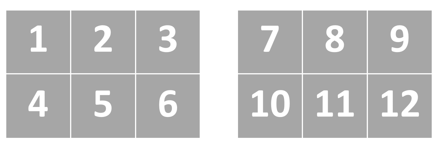
首先,我们讨论一下什么是存储(Storage),什么是视图(View)。
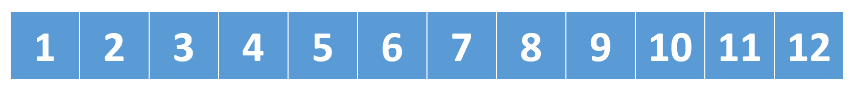
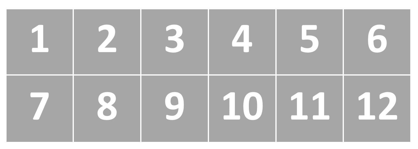
我们可以在读取的时候,读成2行,每行6个。
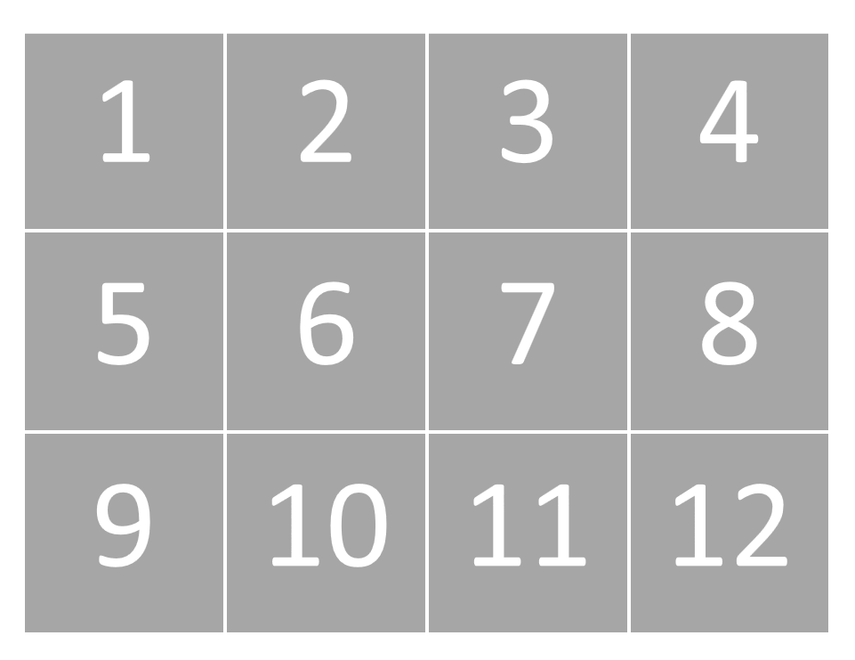
也可以读成3行,每行3个。
甚至可以读成2份,每份2行,每行3个。
无论我们用何种方式读取,不改变的是顺序存储。这就是视图。
改变视图
在讨论什么是存储,什么是视图后。再讨论"改变视图"。
示例代码:
1
2
x = tf.range(1 ,13 ) print(x)
运行结果:
1 tf.Tensor([ 1 2 3 4 5 6 7 8 9 10 11 12], shape=(12,), dtype=int32)
如上述的示例代码和运行结果,在创建一个张量后,张量的默认视图就是只有一行的这种。
通过tf.reshape(x, new_shape),可以将张量的视图任意地合法改变。
接下来我们改变视图。
1 2 3 print(tf.reshape(x,[2 ,6 ])) print(tf.reshape(x,[3 ,4 ])) print(tf.reshape(x,[2 ,2 ,3 ]))
运行结果:
1
2
3
4
5
6
7
8
9
10
11
12
13
tf.Tensor( [[ 1 2 3 4 5 6] [ 7 8 9 10 11 12]], shape=(2, 6), dtype=int32) tf.Tensor( [[ 1 2 3 4] [ 5 6 7 8] [ 9 10 11 12]], shape=(3, 4), dtype=int32) tf.Tensor( [[[ 1 2 3] [ 4 5 6]] [[ 7 8 9] [10 11 12]]], shape=(2, 2, 3), dtype=int32)
当然,需要注意的是合法的改变。比如,这种就不行。
1
2
x = tf.range(1 ,13 ) print(tf.reshape(x,[2 ,2 ,2 ,2 ]))
运行结果:
1
2
3
4
【部分运行结果略】 InvalidArgumentError: Input to reshape is a tensor with 12 values, but the requested shape has 16 [Op:Reshape]
增删维度
我们还可以增加一个长度为1的维度。相当于给原有的数据添加一个新维度的概念,维度长度为1,故数据并不需要改变,仅仅是改变数据的理解方式,因此它其实可以理解为改变视图的一种特殊方式。
通过tf.expand_dims(x, axis)可在指定的axis轴前可以插入一个新的维度。 但如果axis为负数,则表示当前axis维度之后插入一个新的维度。
示例代码:
1
2
3
4
5
6
7
8
9
10
11
12
x = tf.range(1 ,13 ) x = tf.reshape(x,[2 ,2 ,3 ]) print(x) x = tf.reshape(x,[2 ,2 ,3 ]) print(tf.expand_dims(x,axis=0 )) x = tf.reshape(x,[2 ,2 ,3 ]) print(tf.expand_dims(x,axis=1 )) x = tf.reshape(x,[2 ,2 ,3 ]) print(tf.expand_dims(x,axis=-2 ))
运行结果:
1
2
3
4
5
6
7
8
9
10
11
12
13
14
15
16
17
18
19
20
21
22
23
24
25
26
27
28
tf.Tensor( [[[ 1 2 3] [ 4 5 6]] [[ 7 8 9] [10 11 12]]], shape=(2, 2, 3), dtype=int32) tf.Tensor( [[[[ 1 2 3] [ 4 5 6]] [[ 7 8 9] [10 11 12]]]], shape=(1, 2, 2, 3), dtype=int32) tf.Tensor( [[[[ 1 2 3] [ 4 5 6]]] [[[ 7 8 9] [10 11 12]]]], shape=(2, 1, 2, 3), dtype=int32) tf.Tensor( [[[[ 1 2 3]] [[ 4 5 6]]] [[[ 7 8 9]] [[10 11 12]]]], shape=(2, 2, 1, 3), dtype=int32)
有增加长度为1的维度,也有删除长度为1的维度。
通过f.squeeze(x, axis)可在指定的axis轴删除一个长度为1的维度。 如果不指定维度参数axis,即tf.squeeze(x),那么它会默认删除所有长度为1的维度。通常不建议这么做,因为写程序还是需要严谨一些,我们无法非常确信不会误删。
示例代码:
1
2
3
4
x = tf.range(1 ,13 ) x = tf.reshape(x,[1 ,2 ,2 ,3 ]) print(x) print(tf.squeeze(x,axis=0 ))
运行结果:
1
2
3
4
5
6
7
8
9
10
11
12
tf.Tensor( [[[[ 1 2 3] [ 4 5 6]] [[ 7 8 9] [10 11 12]]]], shape=(1, 2, 2, 3), dtype=int32) tf.Tensor( [[[ 1 2 3] [ 4 5 6]] [[ 7 8 9] [10 11 12]]], shape=(2, 2, 3), dtype=int32)
交换维度
之前我们讨论的不会改变张量的存储,但是交换维度会。交换维度有点类似于转置。
示例代码:
1
2
3
4
5
6
7
8
9
10
11
x = tf.range(1 ,13 ) print(x) x = tf.reshape(x,[3 ,4 ]) print(x) x = tf.transpose(x) print(x) x = tf.reshape(x,[12 ]) print(x)
运行结果:
1
2
3
4
5
6
7
8
9
10
11
tf.Tensor([ 1 2 3 4 5 6 7 8 9 10 11 12], shape=(12,), dtype=int32) tf.Tensor( [[ 1 2 3 4] [ 5 6 7 8] [ 9 10 11 12]], shape=(3, 4), dtype=int32) tf.Tensor( [[ 1 5 9] [ 2 6 10] [ 3 7 11] [ 4 8 12]], shape=(4, 3), dtype=int32) tf.Tensor([ 1 5 9 2 6 10 3 7 11 4 8 12], shape=(12,), dtype=int32)
如运行结果所示,通过tf.transpose完成维度交换后,不仅仅改变视图,更改变了存储。
广播机制
现在,我们来讨论广播机制。[[1,2],[3,4],[5,6]],我们发现这个数组可以和[10,20]进行相加。
1
2
3
4
5
a = tf.constant([[1 ,2 ],[3 ,4 ],[5 ,6 ]]) b = tf.constant([10 ,20 ]) print(a) print(b) print(a + b)
运行结果:
1
2
3
4
5
6
7
8
9
tf.Tensor( [[1 2] [3 4] [5 6]], shape=(3, 2), dtype=int32) tf.Tensor([10 20], shape=(2,), dtype=int32) tf.Tensor( [[11 22] [13 24] [15 26]], shape=(3, 2), dtype=int32)
那么,这个是怎么实现的呢?
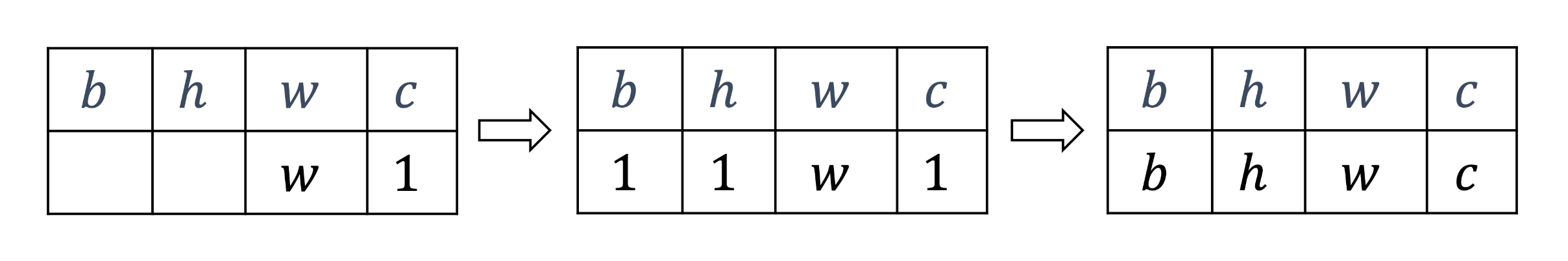
我们把维度从最右边对齐,然后我们把缺失的地方补1。
再把所有维度为1的部分复制为相同的长度。
最后进行运算
比如,在刚刚我例子中,a的形状是(3,2),b的形状是(2)。我们先从最右边对齐,然后不足的地方补1,这时候b的形状是(1,2)。再在所有维度为1的复制到相同的长度,这时候b的形状是(3,2)。最后进行运算。
那么,在TensorFlow中,像这样的两个张量,可以相加吗?
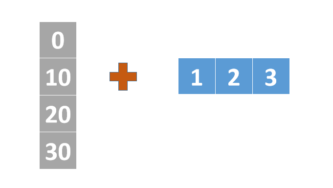
a的形状是(4,1),b的形状是(3)。我们先从最右边对齐,不足的地方部1,则b的形状是(1,3),此时a的形状仍是(4,1)。然后所有的维度为1的复制到相同的长度,注意是所有。所以a的形状是(4,3),b的形状是(4,3)。所以仍可以进行运算。
1
2
3
4
5
a = tf.constant([1 ,2 ,3 ]) b = tf.constant([[0 ],[10 ],[20 ],[30 ]]) print(a) print(b) print(a + b)
运行结果:
1
2
3
4
5
6
7
8
9
10
11
tf.Tensor([1 2 3], shape=(3,), dtype=int32) tf.Tensor( [[ 0] [10] [20] [30]], shape=(4, 1), dtype=int32) tf.Tensor( [[ 1 2 3] [11 12 13] [21 22 23] [31 32 33]], shape=(4, 3), dtype=int32)
但是,需要注意的是,不是所有的都能广播。我们来看一个无法进行广播的例子。
1
2
3
4
5
a = tf.constant([[0 ,1 ,2 ],[3 ,4 ,5 ]]) b = tf.constant([[0 ],[10 ],[20 ],[30 ]]) print(a) print(b) print(a + b)
运行结果:
1
2
3
4
5
6
7
8
9
10
11
12
tf.Tensor( [[0 1 2] [3 4 5]], shape=(2, 3), dtype=int32) tf.Tensor( [[ 0] [10] [20] [30]], shape=(4, 1), dtype=int32) 【部分运行结果略】 InvalidArgumentError: Incompatible shapes: [2,3] vs. [4,1] [Op:AddV2]
我们来分析一下。a的形状是(2,3),b的形状是(4,1)。我们从最右边对齐,不足的地方补1,这一步a和b都不会有变化,然后我们把所有的1都复制成相同的。则a仍是(2,3),b是(4,3)。形状不一样了,自然也就无法进行运算了。
那么?我们为什么要进行广播呢?在《爱情公寓》中,曾小贤只需要在广播台就可以把《你的月亮我的心》这档节目奉献给广大的听众,如果没有广播,那么就需要曾小贤对每位听众都说一遍了,麻烦。
所以,广播的作用:代码更简洁,计算更高效。
数学运算
加减乘除
加、减、乘、除是最基本的数学运算。在TensorFlow中分别通过tf.add()、tf.subtract()、tf.multiply()、tf.divide()函数实现。此外,TensorFlow已经重载了+、−、∗、/运算符,更多的时候,我们一般直接使用运算符来完成加、减、乘、除运算。 除了加减乘除外,常见的运算还有整除和求余,分别通过//和%实现。
示例代码:
1
2
3
4
5
6
7
8
9
10
11
12
13
14
15
16
17
18
a = tf.constant([5 ,6 ]) b = tf.constant(2 ) print(tf.add(a,b)) print(a + b) print(tf.subtract(a,b)) print(a - b ) print(tf.multiply(a,b)) print(a * b) print(tf.divide(a,b)) print(a/b) print(a//b) print(a%b)
运行结果:
1
2
3
4
5
6
7
8
9
10
tf.Tensor([7 8], shape=(2,), dtype=int32) tf.Tensor([7 8], shape=(2,), dtype=int32) tf.Tensor([3 4], shape=(2,), dtype=int32) tf.Tensor([3 4], shape=(2,), dtype=int32) tf.Tensor([10 12], shape=(2,), dtype=int32) tf.Tensor([10 12], shape=(2,), dtype=int32) tf.Tensor([2.5 3. ], shape=(2,), dtype=float64) tf.Tensor([2.5 3. ], shape=(2,), dtype=float64) tf.Tensor([2 3], shape=(2,), dtype=int32) tf.Tensor([1 0], shape=(2,), dtype=int32)
指数运算
乘方通过tf.pow()实现。
1
2
3
4
5
a = tf.constant([5 ,6 ]) b = tf.constant(2 ) print(tf.pow(a,b)) print(a**b)
运行结果:
1
2
tf.Tensor([25 36], shape=(2,), dtype=int32) tf.Tensor([25 36], shape=(2,), dtype=int32)
平方根通过tf.sqrt()实现。
1
2
3
4
5
6
a = tf.constant([5 ,6 ],dtype=tf.float32) b = tf.constant(0.5 ) print(tf.pow(a,b)) print(a**b) print(tf.sqrt(a))
运行结果:
1
2
3
tf.Tensor([2.236068 2.4494898], shape=(2,), dtype=float32) tf.Tensor([2.236068 2.4494898], shape=(2,), dtype=float32) tf.Tensor([2.236068 2.4494898], shape=(2,), dtype=float32)
特别地,对于自然指数e x e^x e x tf.exp(x)实现。
1 2 3 4 5 6 print(tf.exp(1.0 )) print(tf.exp(2.0 )) e = tf.constant(math.e) print(tf.pow(e,1.0 )) print(tf.pow(e,2.0 ))
运行结果:
1
2
3
4
tf.Tensor(2.7182817, shape=(), dtype=float32) tf.Tensor(7.389056, shape=(), dtype=float32) tf.Tensor(2.7182817, shape=(), dtype=float32) tf.Tensor(7.3890557, shape=(), dtype=float32)
对数运算
在TensorFlow中,自然对数log e x \log_e^x log e x tf.math.log(x)实现。
1
2
3
4
print(tf.math.log(math.e)) e = tf.constant(math.e) print(tf.math.log(e))
运行结果:
1
2
tf.Tensor(0.99999994, shape=(), dtype=float32) tf.Tensor(0.99999994, shape=(), dtype=float32)
如果希望计算其它底数的对数,可以根据对数的换底公式实现。
log a x = log e x log e a \log_a^x = \frac{\log_e^x}{\log_e^a}
log a x = log e a log e x
如计算log 10 100 \log_{10}^{100} log 1 0 1 0 0
log 10 100 = log e 100 log e 10 \log_{10}^{100} = \frac{\log_e^{100}}{\log_e^{10}}
log 1 0 1 0 0 = log e 1 0 log e 1 0 0
示例代码:
1 print(tf.math.log(100.0)/tf.math.log(10.0))
运行结果:
1 tf.Tensor(2.0, shape=(), dtype=float32)
张量相乘
在TensorFlow中,矩阵相乘可以通过运算符@实现,也可以通过tf.matmul(a,b)函数实现。
1
2
3
4
5
6
7
8
a = tf.constant([[1 ,2 ],[3 ,4 ],[5 ,6 ]]) b = tf.constant([[1 ],[3 ]]) print(a) print(b) print(a @ b) print(tf.matmul(a,b))
运行结果:
1
2
3
4
5
6
7
8
9
10
11
12
13
14
15
tf.Tensor( [[1 2] [3 4] [5 6]], shape=(3, 2), dtype=int32) tf.Tensor( [[1] [3]], shape=(2, 1), dtype=int32) tf.Tensor( [[ 7] [15] [23]], shape=(3, 1), dtype=int32) tf.Tensor( [[ 7] [15] [23]], shape=(3, 1), dtype=int32)
在大二的课程中,有关于矩阵相乘的条件:A \bold{A} A m ∗ s m*s m ∗ s B \bold{B} B s ∗ n s*n s ∗ n A \bold{A} A B \bold{B} B A \bold{A} A B \bold{B} B A B \bold{AB} A B m ∗ n m*n m ∗ n
在张量中,两个张量能够相乘的条件是:前一个张量的倒数第一个维度的长度和后一个张量的倒数第二个维度长度必须相等。
1
2
3
4
5
6
7
8
a = tf.constant([[[1 ,2 ,3 ],[4 ,5 ,6 ]],[[11 ,12 ,13 ],[14 ,15 ,16 ]]]) b = tf.constant([[[1 ],[2 ],[3 ]],[[4 ],[5 ],[6 ]]]) print(a) print(b) print(a @ b) print(tf.matmul(a,b))
运行结果:
1
2
3
4
5
6
7
8
9
10
11
12
13
14
15
16
17
18
19
20
21
22
23
24
25
26
tf.Tensor( [[[ 1 2 3] [ 4 5 6]] [[11 12 13] [14 15 16]]], shape=(2, 2, 3), dtype=int32) tf.Tensor( [[[1] [2] [3]] [[4] [5] [6]]], shape=(2, 3, 1), dtype=int32) tf.Tensor( [[[ 14] [ 32]] [[182] [227]]], shape=(2, 2, 1), dtype=int32) tf.Tensor( [[[ 14] [ 32]] [[182] [227]]], shape=(2, 2, 1), dtype=int32)
矩阵相乘函数同样支持自动广播机制。
1 2 3 4 5 6 7 8 a = tf.constant([[[1 ,2 ,3 ],[4 ,5 ,6 ]],[[11 ,12 ,13 ],[14 ,15 ,16 ]]]) b = tf.constant([[1 ],[2 ],[3 ]]) print(a) print(b) print(a @ b) print(tf.matmul(a,b))
运行结果:
1 2 3 4 5 6 7 8 9 10 11 12 13 14 15 16 17 18 19 20 21 22 tf.Tensor( [[[ 1 2 3] [ 4 5 6]] [[11 12 13] [14 15 16]]], shape=(2, 2, 3), dtype=int32) tf.Tensor( [[1] [2] [3]], shape=(3, 1), dtype=int32) tf.Tensor( [[[14] [32]] [[74] [92]]], shape=(2, 2, 1), dtype=int32) tf.Tensor( [[[14] [32]] [[74] [92]]], shape=(2, 2, 1), dtype=int32)
张量的比较
为了计算分类任务的准确率等指标,一般需要将预测结果和真实标签比较,统计比较结果中正确的数量来计算准确率。
例如,现在有100个样本的预测结果,我先通过tf.nn.softmax(),再通过tf.argmax()获取预测类别。
1 2 3 4 5 6 7 8 out = tf.random.normal([100 ,10 ]) print(out.shape) out = tf.nn.softmax(out, axis=1 ) print(out.shape) pred = tf.argmax(out, axis=1 ) print(pred)
运行结果:
1 2 3 4 5 6 (100, 10) (100, 10) tf.Tensor( [1 6 2 4 0 7 6 0 3 2 5 6 0 2 3 9 2 6 7 3 6 9 3 5 2 1 4 7 8 7 2 4 9 7 7 0 8 5 6 6 1 6 0 4 4 6 1 5 0 1 0 4 6 4 0 0 4 2 5 8 1 3 9 2 3 9 6 9 9 0 7 9 4 7 8 4 1 7 5 1 6 6 1 2 7 7 4 8 5 8 4 3 4 8 8 2 5 1 5 8], shape=(100,), dtype=int64)
那么,我们怎么比较预测值和真实值呢?
或
两者等价。
示例代码:
1 2 3 y = tf.random.uniform([100 ],dtype=tf.int64,maxval=10 ) out = tf.equal(pred,y) print(out)
运行结果:
1 2 3 4 5 6 7 8 9 10 tf.Tensor( [False False True False False False False False False False True False False False False False True True False False False False False False False False False True False False True False False False False False False False False False False False False False False False True True False True False True False False False False False True False False False False False False False False False False False False True False False False True True False False False False False False False True False False False False False False False False True False True False False False False False], shape=(100,), dtype=bool)
那么,怎么统计准确率?
1 2 3 out = tf.cast(out, dtype=tf.float32) correct = tf.reduce_sum(out)/(len(out)) print(correct)
运行结果:
1 tf.Tensor(0.17, shape=(), dtype=float32)
关于tf.reduce_sum(),我们会在下一小节做详细的讨论。
常用比较函数总结
函数
比较逻辑
tf.math.greater
a > b a > b a > b
tf.math.less
a < b a < b a < b
tf.math.equal 或 tf.math.equal(a, b)
a = = b a == b a = = b
tf.math.not_equal
a ≠ b a \neq b a = b
tf.math.greater_equal
a ≥ b a \geq b a ≥ b
tf.math.less_equal
a ≤ b a \leq b a ≤ b
tf.math.is_nan
a a a
数据统计
向量范数
向量范数(Vector Norm)是描述向量"长度"的一种度量方法,常见的向量范数有:
L1范数,向量x \bold{x} x
∣ ∣ x ∣ ∣ 1 = ∑ i ∣ x i ∣ ||\bold{x}||_1 = \sum_{i}|x_i| ∣ ∣ x ∣ ∣ 1 = i ∑ ∣ x i ∣
L2范数,向量x \bold{x} x
∣ ∣ x ∣ ∣ 2 = ∑ i x i 2 ||\bold{x}||_2 = \sqrt{\sum_{i}x_i^2} ∣ ∣ x ∣ ∣ 2 = i ∑ x i 2
∞ \infty ∞ x \bold{x} x
∣ ∣ x ∣ ∣ ∞ = max i ( ∣ x i ∣ ) ||\bold{x}||_{\infty} = \max_i(|x_i|) ∣ ∣ x ∣ ∣ ∞ = i max ( ∣ x i ∣ )
对于矩阵和张量,同样可以利用向量范数的计算公式,等价于将矩阵和张量打平成向量后计算。
在TensorFlow中,可以通过tf.norm(x, ord)求解张量的L1、L2、∞ \infty ∞ ord指定为1、2时计算L1、L2范数,指定为np.inf时计算∞ \infty ∞
示例代码:
1 2 3 4 5 x = tf.constant([[1.0 ],[2.0 ],[3.0 ]]) print(tf.norm(x,ord=1 )) print(tf.norm(x,ord=2 )) print(tf.norm(x,ord=np.inf))
运行结果:
1 2 3 tf.Tensor(6.0, shape=(), dtype=float32) tf.Tensor(3.7416575, shape=(), dtype=float32) tf.Tensor(3.0, shape=(), dtype=float32)
最值、均值、和
通过tf.reduce_max()、tf.reduce_min()、tf.reduce_mean()、tf.reduce_sum()函数可以求解张量在某个维度上的最大、最小、均值、和,也可以求全局最大、最小、均值、和。 当不指定axis参数时,tf.reduce_*函数求解的就是全局的最大、最小、均值、和。
tf.reduce_max()
1 2 3 4 x = tf.constant([[1 ,2 ],[3 ,4 ],[5 ,6 ],[7 ,8 ]]) print(x) print(tf.reduce_max(x,axis=1 )) print(tf.reduce_max(x))
运行结果:
1 2 3 4 5 6 7 tf.Tensor( [[1 2] [3 4] [5 6] [7 8]], shape=(4, 2), dtype=int32) tf.Tensor([2 4 6 8], shape=(4,), dtype=int32) tf.Tensor(8, shape=(), dtype=int32)
tf.reduce_min()
1 2 3 4 x = tf.constant([[1 ,2 ],[3 ,4 ],[5 ,6 ],[7 ,8 ]]) print(x) print(tf.reduce_min(x,axis=1 )) print(tf.reduce_min(x))
运行结果:
1 2 3 4 5 6 7 tf.Tensor( [[1 2] [3 4] [5 6] [7 8]], shape=(4, 2), dtype=int32) tf.Tensor([1 3 5 7], shape=(4,), dtype=int32) tf.Tensor(1, shape=(), dtype=int32)
tf.reduce_mean()
1 2 3 4 x = tf.constant([[1.0 ,2.0 ],[3.0 ,4.0 ],[5.0 ,6.0 ],[7.0 ,8.0 ]]) print(x) print(tf.reduce_mean(x,axis=1 )) print(tf.reduce_mean(x))
运行结果:
1 2 3 4 5 6 7 tf.Tensor( [[1. 2.] [3. 4.] [5. 6.] [7. 8.]], shape=(4, 2), dtype=float32) tf.Tensor([1.5 3.5 5.5 7.5], shape=(4,), dtype=float32) tf.Tensor(4.5, shape=(), dtype=float32)
特别注意:
此时定义的张量x \bold{x} x
tf.reduce_sum()
1 2 3 4 x = tf.constant([[1 ,2 ],[3 ,4 ],[5 ,6 ],[7 ,8 ]]) print(x) print(tf.reduce_sum(x,axis=1 )) print(tf.reduce_sum(x))
运行结果:
1 2 3 4 5 6 7 tf.Tensor( [[1 2] [3 4] [5 6] [7 8]], shape=(4, 2), dtype=int32) tf.Tensor([ 3 7 11 15], shape=(4,), dtype=int32) tf.Tensor(36, shape=(), dtype=int32)
数据限幅
我们知道在深度学习中应用最广泛的一个激活函数是ReLU。
r e l u ( x ) = { x for x ≥ 0 0 for x < 0 relu(x) = \begin{cases}
x & \text{for } x \ge 0 \\
0 & \text{for } x < 0
\end{cases}
r e l u ( x ) = { x 0 for x ≥ 0 for x < 0
我们可以通过tf.nn.relu实现ReLU函数,也可以用if-else实现。还有一种方法,我们通过tf.maximum(x,a)和tf.minimum(x,b)的组合进行限幅。
我们通过tf.maximum(x, a)实现数据的下限幅,即x ∈ [ a , + ∞ ) x \in [a,+\infty) x ∈ [ a , + ∞ ) ReLU函数。
示例代码:
1 2 3 4 def relu (x) : return tf.maximum(x,0 ) print(relu([-1 ,0 ,1 ]))
运行结果:
1 tf.Tensor([0 0 1], shape=(3,), dtype=int32)
此外,我们还可以通过可以通过tf.minimum(x,a)实现数据的上限幅,即x ∈ ( − ∞ , a ] x \in (- \infty,a] x ∈ ( − ∞ , a ]
通过组合tf.maximum(x,a)和tf.minimum(x,b)可以实现同时对数据的上下边界限幅。
1 2 3 x = tf.constant([-2 ,-1 ,0 ,1 ,2 ]) print(tf.minimum(tf.maximum(x,-1 ),1 ))
运行结果:
1 tf.Tensor([-1 -1 0 1 1], shape=(5,), dtype=int32)
更方便地,我们可以使用tf.clip_by_value()函数实现上下限幅。
1 2 3 x = tf.constant([-2 ,-1 ,0 ,1 ,2 ]) print(tf.clip_by_value(x,-1 ,1 ))
运行结果:
1 tf.Tensor([-1 -1 0 1 1], shape=(5,), dtype=int32)
数据集的操作
随机打散
通过Dataset.shuffle(buffer_size)工具可以设置Dataset对象随机打散数据之间的顺序。buffer_size参数指定缓冲池的大小,一般设置为一个较大的常数即可。
1 2 3 4 5 6 7 8 9 10 11 12 13 14 15 16 17 import tensorflow as tffrom tensorflow.keras import datasets(x_train, y_train), (x_test, y_test) = datasets.mnist.load_data() train_db = tf.data.Dataset.from_tensor_slices((x_train, y_train)) for step, (x, y) in enumerate(train_db): if step > 10 : break print(y) print('\n' * 3 ) train_db = train_db.shuffle(10000 ) for step, (x, y) in enumerate(train_db): if step > 10 : break print(y)
运行结果:
1 2 3 4 5 6 7 8 9 10 11 12 13 14 15 16 17 18 19 20 21 22 23 24 25 26 tf.Tensor(5, shape=(), dtype=uint8) tf.Tensor(0, shape=(), dtype=uint8) tf.Tensor(4, shape=(), dtype=uint8) tf.Tensor(1, shape=(), dtype=uint8) tf.Tensor(9, shape=(), dtype=uint8) tf.Tensor(2, shape=(), dtype=uint8) tf.Tensor(1, shape=(), dtype=uint8) tf.Tensor(3, shape=(), dtype=uint8) tf.Tensor(1, shape=(), dtype=uint8) tf.Tensor(4, shape=(), dtype=uint8) tf.Tensor(3, shape=(), dtype=uint8) tf.Tensor(2, shape=(), dtype=uint8) tf.Tensor(1, shape=(), dtype=uint8) tf.Tensor(8, shape=(), dtype=uint8) tf.Tensor(7, shape=(), dtype=uint8) tf.Tensor(2, shape=(), dtype=uint8) tf.Tensor(8, shape=(), dtype=uint8) tf.Tensor(4, shape=(), dtype=uint8) tf.Tensor(5, shape=(), dtype=uint8) tf.Tensor(9, shape=(), dtype=uint8) tf.Tensor(2, shape=(), dtype=uint8) tf.Tensor(3, shape=(), dtype=uint8)
批训练
为了利用显卡的并行计算能力,一般在网络的计算过程中会同时计算多个样本,我们把这种训练方式叫做批训练,其中一个批中样本的数量叫做Batch Size。为了一次能够从Dataset中产生Batch Size数量的样本,需要设置Dataset为批训练方式,实现如下:
1 2 # 设置批训练,batch size 为 128 train_db = train_db.batch(128)
其中128为Batch Size参数,即一次并行计算128个样本的数据。Batch Size一般根据用户的GPU显存资源来设置,当显存不足时,可以适量减少Batch Size来减少算法的显存使用量。
.batch()方法后,我们并不需要手动进行循环遍历,直接传入模型的.fit()方法即可。
用Batch Size的话,还有助于TensorFlow自动回收内存。在CPU训练中,也非常有帮助。
预处理
Dataset对象通过提供map(func)工具函数,可以非常方便地调用用户自定义的预处理逻辑,它实现在func函数里。
1 2 3 4 5 6 7 8 9 10 11 12 13 14 15 16 17 18 19 20 21 22 23 24 25 26 27 28 29 30 31 import tensorflow as tffrom tensorflow.keras import datasetsdef preprocess (xv, yv) : """ :param xv: :param yv: :return: """ xv = tf.cast(xv, dtype=tf.float32) / 255.0 yv = tf.one_hot(tf.cast(yv, dtype=tf.int32), depth=10 ) return xv, yv (x_train, y_train), (x_test, y_test) = datasets.mnist.load_data() train_db = tf.data.Dataset.from_tensor_slices((x_train, y_train)) for step, (x, y) in enumerate(train_db): if step > 10 : break print(y) print('\n' * 3 ) train_db = train_db.map(preprocess) for step, (x, y) in enumerate(train_db): if step > 10 : break print(y)
运行结果:
1 2 3 4 5 6 7 8 9 10 11 12 13 14 15 16 17 18 19 20 21 22 23 24 25 26 tf.Tensor(5, shape=(), dtype=uint8) tf.Tensor(0, shape=(), dtype=uint8) tf.Tensor(4, shape=(), dtype=uint8) tf.Tensor(1, shape=(), dtype=uint8) tf.Tensor(9, shape=(), dtype=uint8) tf.Tensor(2, shape=(), dtype=uint8) tf.Tensor(1, shape=(), dtype=uint8) tf.Tensor(3, shape=(), dtype=uint8) tf.Tensor(1, shape=(), dtype=uint8) tf.Tensor(4, shape=(), dtype=uint8) tf.Tensor(3, shape=(), dtype=uint8) tf.Tensor([0. 0. 0. 0. 0. 1. 0. 0. 0. 0.], shape=(10,), dtype=float32) tf.Tensor([1. 0. 0. 0. 0. 0. 0. 0. 0. 0.], shape=(10,), dtype=float32) tf.Tensor([0. 0. 0. 0. 1. 0. 0. 0. 0. 0.], shape=(10,), dtype=float32) tf.Tensor([0. 1. 0. 0. 0. 0. 0. 0. 0. 0.], shape=(10,), dtype=float32) tf.Tensor([0. 0. 0. 0. 0. 0. 0. 0. 0. 1.], shape=(10,), dtype=float32) tf.Tensor([0. 0. 1. 0. 0. 0. 0. 0. 0. 0.], shape=(10,), dtype=float32) tf.Tensor([0. 1. 0. 0. 0. 0. 0. 0. 0. 0.], shape=(10,), dtype=float32) tf.Tensor([0. 0. 0. 1. 0. 0. 0. 0. 0. 0.], shape=(10,), dtype=float32) tf.Tensor([0. 1. 0. 0. 0. 0. 0. 0. 0. 0.], shape=(10,), dtype=float32) tf.Tensor([0. 0. 0. 0. 1. 0. 0. 0. 0. 0.], shape=(10,), dtype=float32) tf.Tensor([0. 0. 0. 1. 0. 0. 0. 0. 0. 0.], shape=(10,), dtype=float32)
循环训练
对于Dataset对象,在使用时可以通过
1 2 # 迭代数据集对象,带step参数 for step, (x,y) in enumerate(train_db):
或
1 2 # 迭代数据集对象 for x,y in train_db:
方式进行迭代,每次返回的x和y即为批量样本和标签。这样完成一个Batch的数据训练,叫做一个Step;通过多个step来完成整个训练集的一次迭代,叫做一个Epoch。在实际训练时,通常需要对数据集迭代多个Epoch才能取得较好地训练效果。
1 2 3 4 5 # 训练 Epoch 数 for epoch in range(20): # 迭代 Step 数 for step, (x,y) in enumerate(train_db): # training...
此外,也可以通过设置Dataset对象,使得数据集对象内部遍历多次才会退出,实现如下:
1 2 # 数据集迭代 20 遍才终止 train_db = train_db.repeat(20)
补充操作
最后我们补充几个操作,这些操作可能较少使用,但功能强大。
tf.gathertf.gather_ndtf.boolean_masktf.wheretf.scatter_ndtf.meshgrid
tf.gather
例如,我们现在有七千张MINIST的手写图片。
1 2 3 (x_train, y_train), (x_test, y_test) = mnist.load_data() x = tf.concat([x_train,x_test],axis=0 ) print(x.shape)
运行结果:
现在我们要找出[3,14,15,926]这几张。tf.gather就是针对这个设计的。
使用tf.gather采样多个样本时,表达式类似[3,14,15,926],即每个采样点的索引号。
示例代码:
1 print(tf.gather(x,[3 ,14 ,15 ,926 ],axis=0 ))
运行结果:
1 2 3 4 5 6 7 8 9 10 tf.Tensor( [[[0 0 0 ... 0 0 0] [0 0 0 ... 0 0 0] [0 0 0 ... 0 0 0] 【部分运行结果略】 [0 0 0 ... 0 0 0] [0 0 0 ... 0 0 0] [0 0 0 ... 0 0 0]]], shape=(4, 28, 28), dtype=uint8)
tf.gather_nd
现在我们换一下。我们要提取这些数据:
第4张图片的15行数据
第16张图片的第10行数据
第27张图片的第6行数据
可以通过笨方式,一个一个的手动提取数据。但有更好的办法:tf.gather_nd。
使用tf.gather_nd采样多个样本时,表达式类似[[3,14],[15,9],[26,5]],外层的括号长度为采样样本的个数,内层列表包含了每个采样点的索引坐标。
示例代码:
1 print(tf.gather_nd(x,[[3 ,14 ],[15 ,9 ],[26 ,5 ]]))
运行结果:
1 2 3 4 5 6 7 tf.Tensor( [[ 0 0 0 0 0 0 0 0 0 0 0 0 80 240 251 193 23 0 0 0 0 0 0 0 0 0 0 0] [ 0 0 0 0 0 0 0 0 25 192 226 226 241 252 253 202 252 252 252 252 252 225 0 0 0 0 0 0] [ 0 0 0 0 0 0 0 0 0 0 0 0 0 0 0 0 0 0 0 0 0 0 0 0 0 0 0 0]], shape=(3, 28), dtype=uint8)
tf.boolean_mask
除了可以通过给定索引号的方式采样,还可以通过给定掩码(Mask)的方式进行采样。tf.boolean_mask(x, mask, axis)可以在axis轴上根据mask方案进行采样。
1 2 3 4 5 (x_train, y_train), (x_test, y_test) = mnist.load_data() x = x_train[:4 ] print(x.shape) mask = [True , False , False , True ] print(tf.boolean_mask(x, mask, axis=0 ))
运行结果:
1 2 3 4 5 6 7 8 9 10 11 (4, 28, 28) tf.Tensor( [[[0 0 0 ... 0 0 0] [0 0 0 ... 0 0 0] [0 0 0 ... 0 0 0] 【部分运行结果略】 [0 0 0 ... 0 0 0] [0 0 0 ... 0 0 0] [0 0 0 ... 0 0 0]]], shape=(2, 28, 28), dtype=uint8)