比赛链接
JPX Tokyo Stock Exchange Prediction
https://www.kaggle.com/competitions/jpx-tokyo-stock-exchange-prediction
数据
数据概览
1 | +--data_specifications |
data_specifications
对数据的描述(列名含义、数据解释等)stock_list.csv
股票列表jpx_tokyo_market_prediction
JPX的赛题属于"Code Competition",jpx_tokyo_market_prediction是在Linux系统下的运行环境。example_test_files
样例数据supplemental_files
可以理解为验证集数据train_files
训练集数据
train_files
我们重点关注train_files中的文件。
1 | +--train_files |
financials.csv
financials.csv,上市公司的财报数据。
查看financials.csv中的内容,示例代码:
1 | financials = pd.read_csv('../jpxd/train_files/financials.csv') |
运行结果:
1 | DisclosureNumber DateCode Date SecuritiesCode DisclosedDate DisclosedTime DisclosedUnixTime TypeOfDocument CurrentPeriodEndDate TypeOfCurrentPeriod CurrentFiscalYearStartDate CurrentFiscalYearEndDate NetSales OperatingProfit OrdinaryProfit Profit EarningsPerShare TotalAssets Equity EquityToAssetRatio BookValuePerShare ResultDividendPerShare1stQuarter ResultDividendPerShare2ndQuarter ResultDividendPerShare3rdQuarter ResultDividendPerShareFiscalYearEnd ResultDividendPerShareAnnual ForecastDividendPerShare1stQuarter ForecastDividendPerShare2ndQuarter ForecastDividendPerShare3rdQuarter ForecastDividendPerShareFiscalYearEnd ForecastDividendPerShareAnnual ForecastNetSales ForecastOperatingProfit ForecastOrdinaryProfit ForecastProfit ForecastEarningsPerShare ApplyingOfSpecificAccountingOfTheQuarterlyFinancialStatements MaterialChangesInSubsidiaries ChangesBasedOnRevisionsOfAccountingStandard ChangesOtherThanOnesBasedOnRevisionsOfAccountingStandard ChangesInAccountingEstimates RetrospectiveRestatement NumberOfIssuedAndOutstandingSharesAtTheEndOfFiscalYearIncludingTreasuryStock NumberOfTreasuryStockAtTheEndOfFiscalYear AverageNumberOfShares |
在市场不存在内幕交易的情况下,如果财报不及预期,可能在财报发布后会有一段时间的反应。但我们很难判断财报是否达到预期,我们不会过多关注该数据。
options.csv
options.csv,期权数据。
期权确实有一个功能:价格发现。
但是,根据东京证券交易所的资料,没有个股期权,也没有行业指数期权,东京证券交易所的期权的标的资产都是和宏观有关的指数,或者大宗商品。
也就是说,东京证券交易所的期权,不具有对于个股或行业的价格发现功能。
即,认为期权数据的帮助有限。
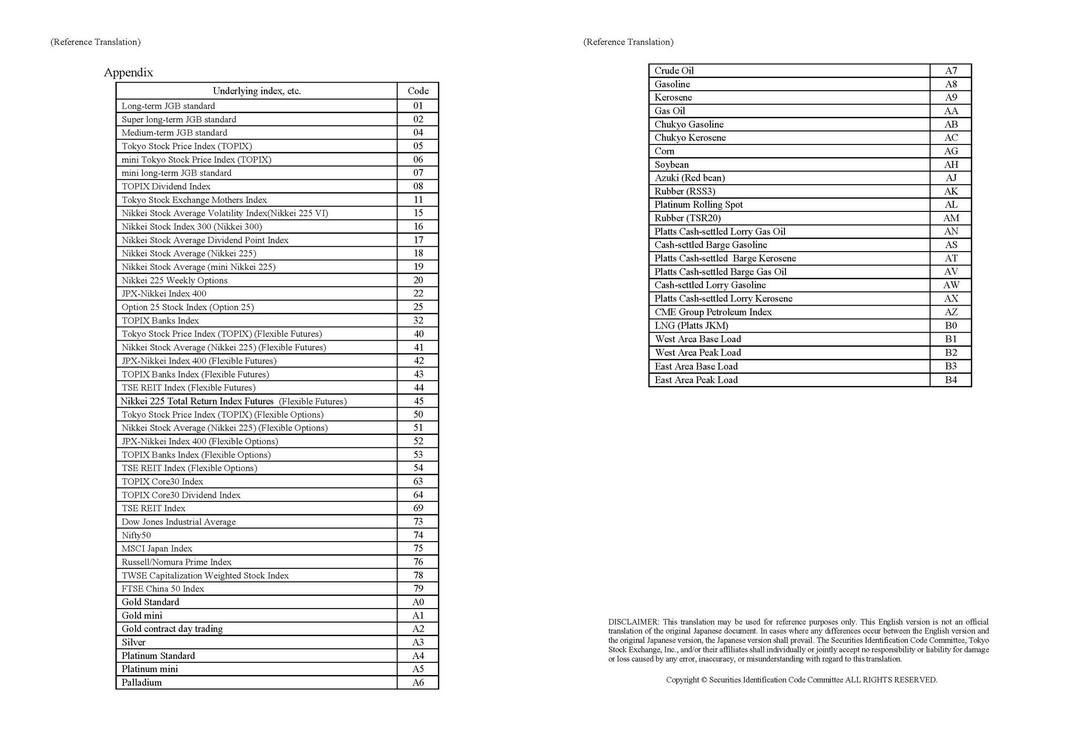
东京证券交易所链接:https://www.jpx.co.jp/english/sicc/regulations/b5b4pj0000023mqo-att/(HP)sakimono20220208-e.pdf
secondary_stock_prices.csv
东京证券交易所市场二部的股票数据。
stock_prices.csv
stock_prices.csv,股票价格数据。
字段
查看stock_prices.csv中的内容,会发现是日线数据。示例代码:
1 | stock_prices = pd.read_csv('../jpxd/train_files/stock_prices.csv') |
运行结果:
1 | RowId Date SecuritiesCode Open High Low Close Volume AdjustmentFactor ExpectedDividend SupervisionFlag Target |
RowId,每一行的唯一标识。Date,日期。SecuritiesCode,证券代码。Open、High、Low、Close、Volume,分别是开盘价、最高价、最低价、收盘价、成交量。AdjustmentFactor,调整因子(复权因子)。
拆股、合股、配股、送股和派息等,都可能会影响调整因子。
举个例子,例如原本股价是每股100,拆成10股后,每股可能是10,同时交易量会是原来的10倍。ExpectedDividend:除权日的预期股息价值,该价值记录于除息日前2个工作日。SupervisionFlag:被监管,或者即将退市。(类似于国内的风险警示,ST。)Target;目标值,即标签。
Target的计算方法如下:
- 表示第支股票在时刻的收盘价。
- 表示第支股票在时刻的收盘价。
- 表示第支股票在时刻的收益,即
Target
即日的Target,是这一天的涨跌幅;是假设在日以收盘价买入,在日以收盘价卖出,这时候的收益。
时间范围
stock_prices.csv在两处有:
train_files/stock_prices.csvsupplemental_files/stock_prices.csv
查看两份数据的时间范围。示例代码:
1 | train_files_stock_prices = pd.read_csv('../jpxd/train_files/stock_prices.csv') |
运行结果:
1 | train的起始时间:2017-01-04,train的结束时间:2021-12-03 |
trades.csv
trades.csv,市场运行周报。
每一个板块,在某一周的运行情况。
我认为该部分的数据,没有帮助。
查看trades.csv,示例代码:
1 | trades = pd.read_csv('../jpxd/train_files/trades.csv') |
运行结果:
1 | Date StartDate EndDate Section TotalSales TotalPurchases TotalTotal TotalBalance ProprietarySales ProprietaryPurchases ProprietaryTotal ProprietaryBalance BrokerageSales BrokeragePurchases BrokerageTotal BrokerageBalance IndividualsSales IndividualsPurchases IndividualsTotal IndividualsBalance ForeignersSales ForeignersPurchases ForeignersTotal ForeignersBalance SecuritiesCosSales SecuritiesCosPurchases SecuritiesCosTotal SecuritiesCosBalance InvestmentTrustsSales InvestmentTrustsPurchases InvestmentTrustsTotal InvestmentTrustsBalance BusinessCosSales BusinessCosPurchases BusinessCosTotal BusinessCosBalance OtherInstitutionsSales OtherInstitutionsPurchases OtherInstitutionsTotal OtherInstitutionsBalance InsuranceCosSales InsuranceCosPurchases InsuranceCosTotal InsuranceCosBalance CityBKsRegionalBKsEtcSales CityBKsRegionalBKsEtcPurchase CityBKsRegionalBKsEtcTotal CityBKsRegionalBKsEtcBalance TrustBanksSales TrustBanksPurchases TrustBanksTotal TrustBanksBalance OtherFinancialInstitutionsSales OtherFinancialInstitutionsPurchases OtherFinancialInstitutionsTotal OtherFinancialInstitutionsBalance |
题外话
根据东京证券交易所官方资料,是2022年4月4日,重新对市场进行了划分。然后才有Growth Market、Prime Market和Standard Market三个市场。但是根据trades.csv,我们看到在2021年11月,已经有了Growth Market、Prime Market和Standard Market三个市场的运行周报数据。
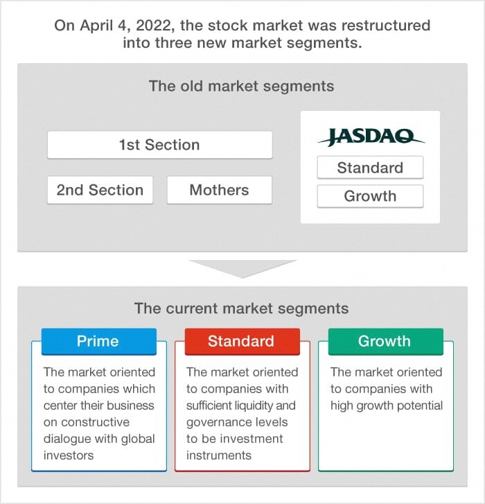
东京证券交易所链接:https://www.jpx.co.jp/english/equities/market-restructure/market-segments/index.html
stock_list.csv
stock_list.csv,股票的基本信息。
查看stock_list.csv,示例代码:
1 | stock_list = pd.read_csv('../jpxd/stock_list.csv') |
运行结果:
1 | SecuritiesCode EffectiveDate Name Section/Products NewMarketSegment 33SectorCode 33SectorName 17SectorCode 17SectorName NewIndexSeriesSizeCode NewIndexSeriesSize TradeDate Close IssuedShares MarketCapitalization Universe0 |
33SectorCode、33SectorName17SectorCode、17SectorName
两种行业分类方式。根据东京证券交易所资料,"33"这个行业分类方式更精细化,"17"是基于"33"的进行的划分。
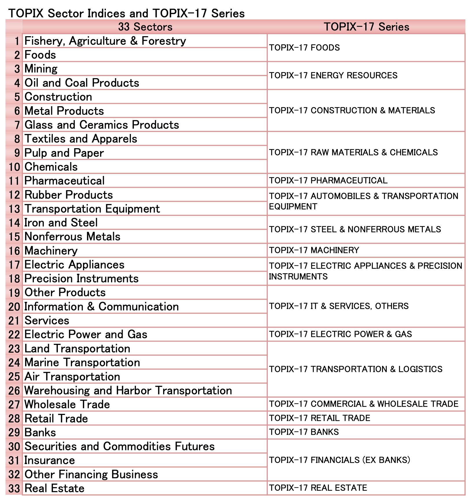
东京证券交易所链接地址:https://www.jpx.co.jp/english/markets/indices/line-up/files/e_fac_13_sector.pdf
不会出现类似于下图的情况,两种行业分类彼此存在相同的股票和不同的股票。

NewIndexSeriesSizeCode、NewIndexSeriesSize
该部分表示的是某只股票是否属于某一个指数的成分股。
不同的指数对于其成份股有不同要求,所以该部分其实能反应股票的某些特征。
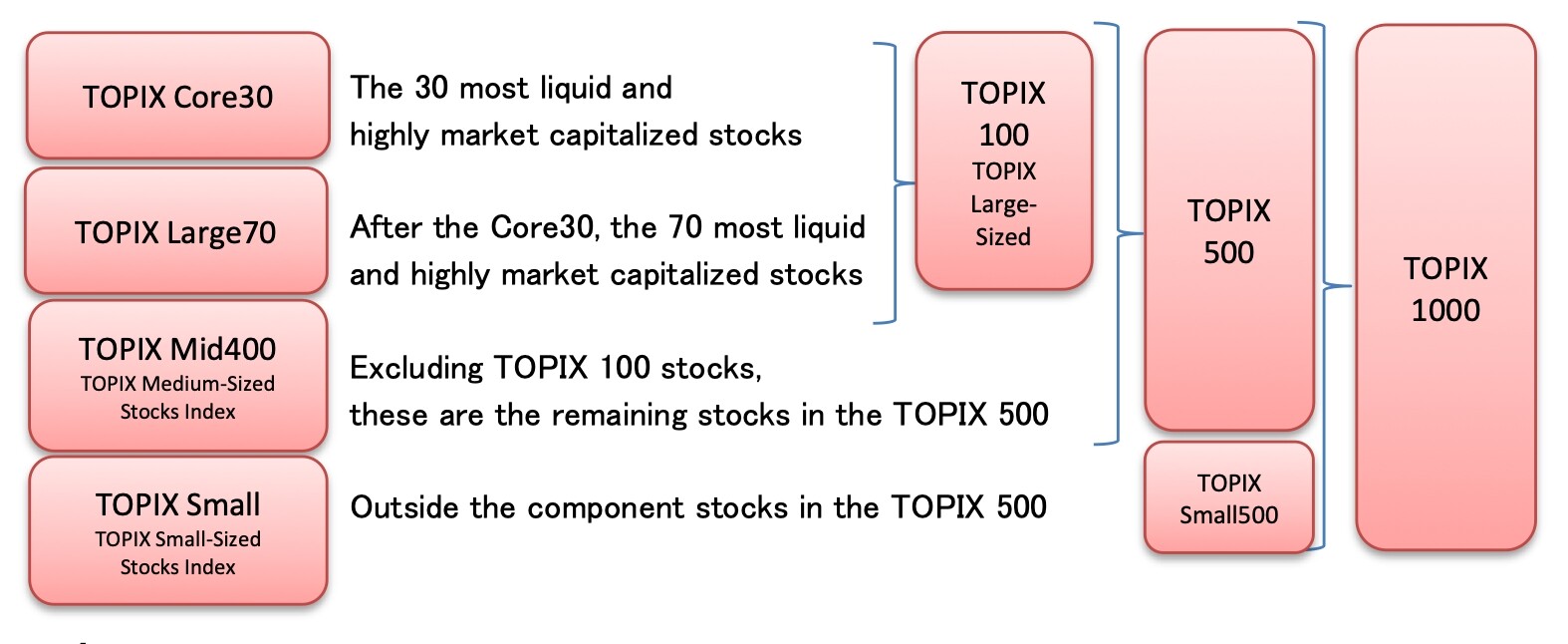
东京证券交易所链接地址:https://www.jpx.co.jp/english/markets/indices/line-up/files/e_fac_12_size.pdf
评分
投资组合
虽然在数据集中有target,但我们要做的并不是预测target,即这不是一个回归问题。
我们需要根据在日对给出的两千只股票进行排序,然后在日做多前200只,做空后200只,并在日进行平仓;在做多和做空的过程中,根据排序对进行加权。
所以整个过程,构成了一个投资组合,最后衡量投资组合的夏普比率。
夏普比率
什么是夏普比率
概述
夏普比率,衡量额外承受的每一单位风险所获得的额外收益。
多个版本的夏普比率
1966年,威廉·F·夏普提出了第一个版本的夏普比率。如下:
其中是资产收益,是无风险收益。
1994年,威廉·F·夏普对第一个版本的夏普比率进行了修改,提出了第二个版本的夏普比率,如下:
在第二个版本中,如果在整个期间是一个恒定的值,则。
还有很多版本的夏普比率。
- 采用的不是无风险收益率,而是某一种有风险的收益率(例如股票指数),将其作为基准收益率。
- 完全不考虑无风险收益率
(在东京证券交易所的比赛中,即是如此。) - 还有些,采用的不是标准差,而是样本标准差。
这些都是在行业具体应用过程中,根据实际情况的"魔改"。
例子
在比赛中的应用
根据东京证券交易所的资料,其在计算夏普比率的时候,没有考虑无风险收益率(基准收益率)。
具体计算过程如下:
- 计算股票的收益率。
- 计算某一天,做多前200只的收益。
- 计算某一天,做空后200只的收益。
- 计算某一天的总收益。
- 计算夏普比率(不考虑无风险收益率)。
计算股票的收益率
其中是第只股票在第天的收盘价,是第只股票在第这一天的收盘价。
即,在日做决策,在日以收盘价做多或做空,在日以收盘价平仓,表示的投资这只股票的收益。
做多前200只
对于排序前200支的股票进行做多,权重服从一个的线性函数,第一个权重为,第二个权重为,第三个权重为,以此类推,最后除以线性函数的均值。
做空后200只
对于排序200只的股票进行做空,权重服从一个的线性函数,倒数一个权重为,倒数二个权重为,倒数三个权重为,以此类推,最后除以均值。
计算每天总回报
因为是做空后200只股票,所以在计算总回报时,应该减去。
计算夏普比率
总收益率的时间序列的平均值,除以,总收益率的时间序列的标准差,不考虑无风险收益率,也不把日经指数作为基准收益率。
实现代码
1 | import numpy as np |
缺失值(停牌)
为什么会有缺失值
在股票日线数据中,如果存在缺失值,一般是因为股票停牌了(不排除交易所自身故障)。
是否存在缺失值
判断哪些列包含缺失值
如果该列存在缺失值则返回True,反之False。示例代码:
1 | stock_prices = pd.concat([train_files_stock_prices, supplemental_files_stock_prices], axis=0) |
运行结果:
1 | RowId False |
统计每列缺失值的数量
统计每列缺失值的数量,示例代码:
1 | stock_prices.isnull().sum() |
运行结果:
1 | RowId 0 |
查看缺失值
查看Open为空的行
查看Open为空的行,示例代码:
1 | stock_prices[stock_prices.Open.isnull()] |
运行结果:
1 | RowId Date SecuritiesCode Open High Low Close Volume AdjustmentFactor ExpectedDividend SupervisionFlag Target |
查看2020-10-01这一天
查看2020-10-01这一天,示例代码:
1 | stock_prices[stock_prices.Date == '2020-10-01'].isnull().sum() |
运行结果:
1 | RowId 0 |
我们看到,这一天有很多股票都有缺失值。因为在这一天,东京证券交易所发生了故障。

缺失值处理
多种处理方法
在《机器学习实战方法(Python):特征工程-1.特征预处理》,我们讨论过如何填补缺失值。在技术上:对于连续型,可以使用均值或者中位数;对于离散型,可以使用众数。
在本文,因为缺失的原因一般是股票停牌,我认为使用均值或者中位数。都是不恰当的。
建议的处理方法有:
- 不处理
- 直接丢弃停牌期间的数据
- 成交量置为0,开收高低等都采用最近一个交易日的收盘价。
第一种方法
对于第一种方法,不处理。需要特别注意,空值的运算。示例代码:
1 | 1 + 2 + 3 + None |
运行结果:
1 | TypeError: unsupported operand type(s) for +: 'int' and 'NoneType' |
第二种方法
实现
利用dropna,可以去除空值。
示例代码:
1 | stock_prices.dropna(subset=['Open', 'Target'], inplace=True) |
运行结果:
1 | RowId Date SecuritiesCode Open High Low Close Volume AdjustmentFactor ExpectedDividend SupervisionFlag Target |
不建议的原因
但是不建议这种方法。
我们将停牌的数据删除了,在进行滑动窗口处理的时候,会很麻烦。因为我们不好判断是因为停牌导致数据被删;还是因为不是交易日,本就没有数据。
例如,统计第1天到第5天共5个交易日的数据,如果在第3天停牌了,数据又被我们删掉了,而且我们还采取了"直接按顺序找5行"这种粗暴的方式。那么,可能最终统计的是第1天到第6天的数据。
总之,不建议。
第三种方法
思路
成交量置为0,开收高低等都采用最近一个交易日的收盘价。
- 对于"成交量置为0",直接
fillna即可。 - 对于"开收高低等都采用最近一个交易日的收盘价"
- 先进行
groupby - 然后用
ffill,按行,填充收盘价。 - 再分别用
bfill,按列,填充开盘价、最高价以及最低价。
- 先进行
实现
示例代码:
1 | train_files_stock_prices = pd.read_csv('../jpxd/train_files/stock_prices.csv') |
运行结果:
1 | RowId Date SecuritiesCode Open High Low Close Volume AdjustmentFactor ExpectedDividend SupervisionFlag Target |
复权
两种复权
- 前复权(向前复权)
就是保持现有价位不变,将以前的价格缩减。 - 后复权(向后复权)
保持先前的价格不变,而将以后的价格增加。
复权的实现(前复权)
对于价格,乘以复权因子。
对于成交量,除以复权因子。
查看复权前,示例代码:
1 | check_1805 = stock_prices[stock_prices['SecuritiesCode'] == 1805] |
运行结果:
1 | RowId Date SecuritiesCode Open High Low Close Volume AdjustmentFactor ExpectedDividend SupervisionFlag Target |
复权,示例代码:
1 | def generate_adjusted_feature_one_stock(one_stock_df: pd.DataFrame): |
查看复权后,关注AdjustedOpen、AdjustedHigh、AdjustedLow、AdjustedClose和AdjustedVolume,示例代码:
1 | check_1805 = adjusted_stock_prices[adjusted_stock_prices['SecuritiesCode'] == 1805] |
运行结果:
1 | RowId Date SecuritiesCode Open High Low Close Volume AdjustmentFactor ExpectedDividend SupervisionFlag Target CumulativeAdjustmentFactor AdjustedOpen AdjustedHigh AdjustedLow AdjustedClose AdjustedVolume |
争议
有些资料只对价格进行了复权,甚至只对收盘价进行了复权。假如只考虑价格,不考虑量价关系;甚至只考虑收盘价,这种复权方法是OK的。
但是如果要用除收盘价外的其他的价格,要考虑量价关系,必须对成交量进行复权。
探索
市场整体情况
示例代码:
1 | # 删掉一些列 |
1 | import plotly.graph_objects as go |
运行结果:
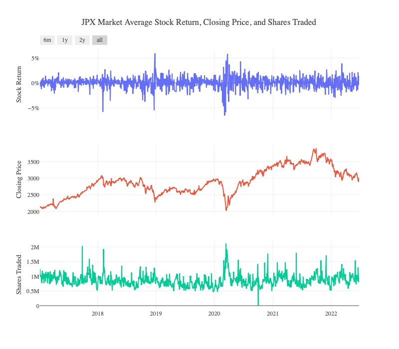
有些资料会说,交易量在逐步下降,但其实是因为他们没有对交易量进行复权。
分行业历年的Return
整理数据:
1 | stock_list=pd.read_csv("../jpxd/stock_list.csv") |
绘制图像:
1 | fig = make_subplots(rows=1, cols=6, shared_yaxes=True) |
运行结果:

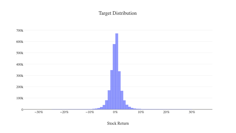
Return的分布
Return的整体分布
示例代码:
1 | fig = go.Figure() |
运行结果:
Return在行业内的分布
示例代码:
1 | pal = ['hsl('+str(h)+',50%'+',50%)' for h in np.linspace(0, 360, 18)] |
运行结果:
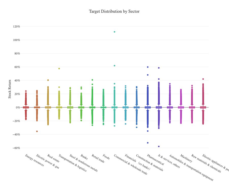
我们直接看数字的话,能更清楚,示例代码:
1 | stock_df_group = stock_df.groupby('SectorName')['Target'].describe() |
运行结果:
1 | count mean std min 25% 50% 75% max |
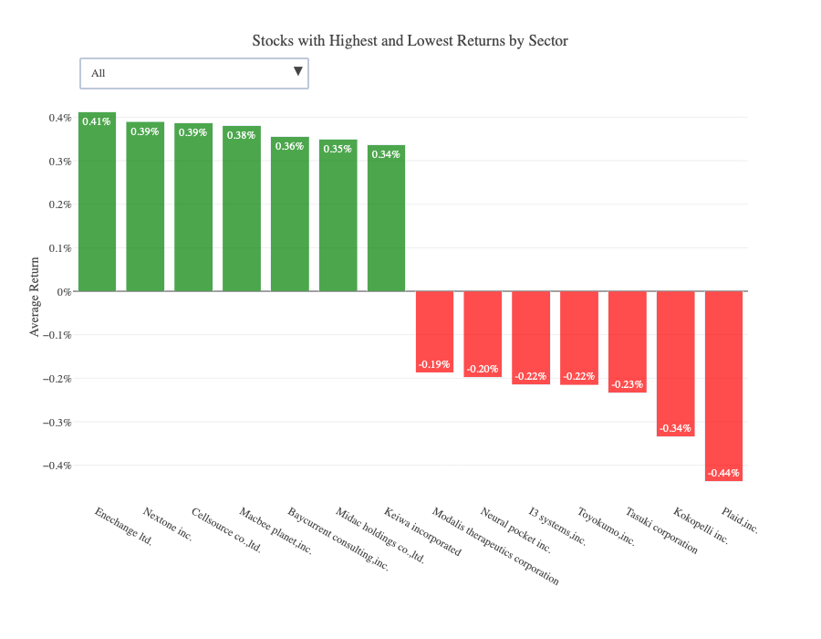
分行业的最高和最低的Return
示例代码:
1 | stock_data=stock_df.groupby('Name')['Target'].mean().mul(100) |
运行结果:
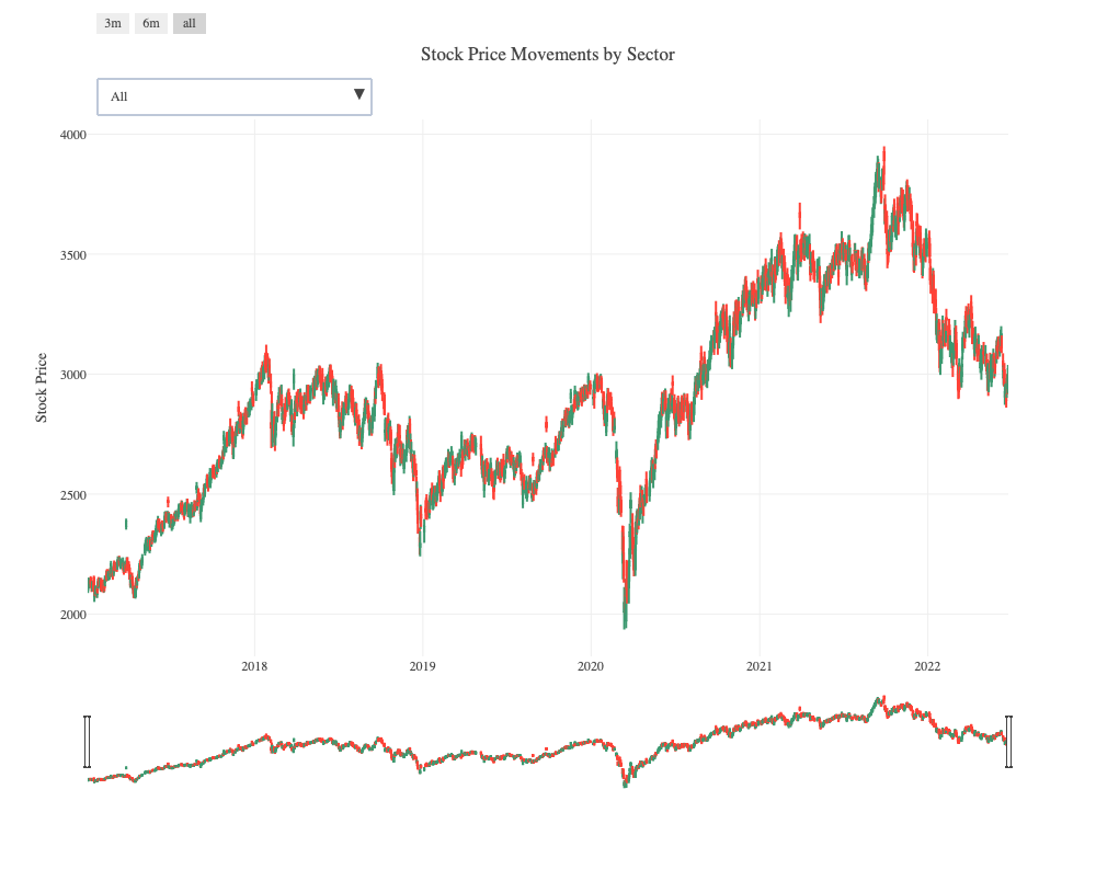
分行业的K线图
示例代码:
1 | stock_date=stock_df.Date.unique() |
运行结果:
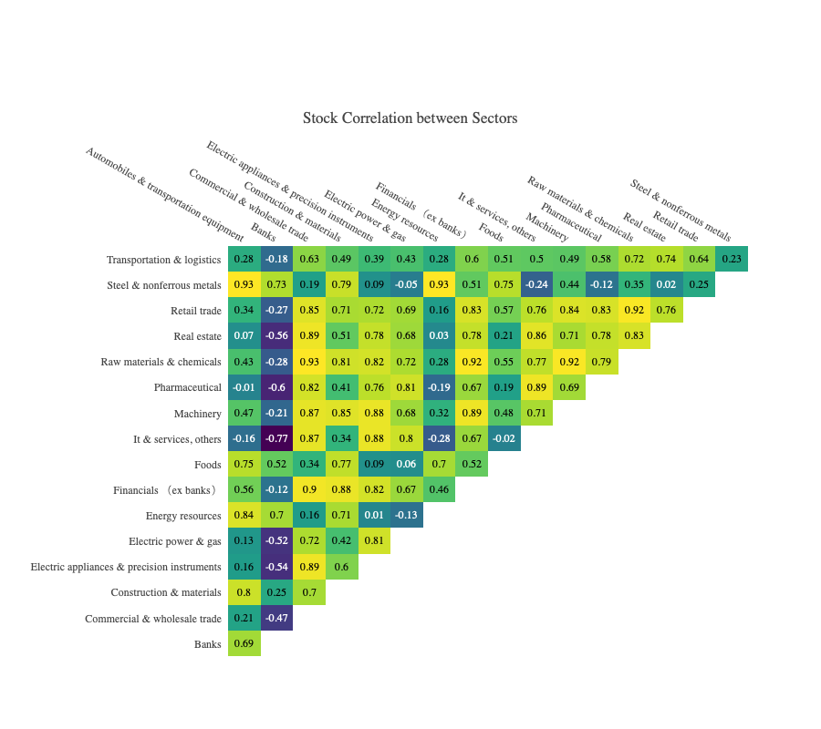
行业间的相关性
示例代码:
1 | import plotly.figure_factory as ff |
运行结果:
补充数据
这个比赛不允许我们ipynb连接互联网,但是允许我们离线补充数据。
jpx-jquants
jpx-jquants概述
jpx-jquants,JPX官方的接口。
获取 Refresh Token
地址:https://api.jquants.com/v1/token/auth_user
请求方式:POST
请求参数:
- Header:不需要
- Body:
- mailaddress:邮箱地址
- password:密码
响应:
- 状态码:200,OK;400,Bad Request;403,Forbidden;500,Internal Server Error。
- 字段:refreshToken
Refresh Token 的有效期是一周。
示例代码:
1 | import requests |
运行结果:
1 | {'refreshToken': 'XXX'} |
获取 ID Token
地址:https://api.jquants.com/v1/token/auth_refresh
请求方式:POST
请求参数:
- Header:不需要
- Query:refreshtoken
响应:
- 状态码:200,OK;400,Bad Request;403,Forbidden;500,Internal Server Error。
- 字段:idToken
ID Token 的有效期是24小时。
示例代码:
1 | import requests |
运行结果:
1 | {'idToken': 'XXX'} |
获取日线数据
地址:https://api.jquants.com/v1/prices/daily_quotes
请求方式:GET
请求参数:
- Header:Authorization,idToken。
- Query:
- code:股票代码。
- from:起始时间,例如,
20210901或2021-09-01。 - to:结束时间,例如,
20210907或2021-09-07。 - date:具体某一天,在没有指定
from和to的时候有效。例如,20210907或2021-09-07。
响应状态吗:200,OK;400,Bad Request;401,Unauthorized;403,Forbidden;413,Payload Too Large;500,Internal Server Error。
响应字段:
Variables | Description | Data type | Remark |
|---|---|---|---|
Date | Date | String | YYYY-MM-DD |
Code | Issue code | String | |
Open | Open Price (before adjustment) | Number | |
High | High price (before adjustment) | Number | |
Low | Low price (before adjustment) | Number | |
Close | Close price (before adjustment) | Number | |
Volume | Trading volume (before Adjustment) | Number | |
TurnoverValue | Trading value | Number | |
AdjustmentFactor | Adjustment factor | Number | In the case of a two-for-one stock split, "0.5" will be set in the record on the ex-rights date. |
AdjustmentOpen | Adjusted open price | Number | ※1 |
AdjustmentHigh | Adjusted high price | Number | ※1 |
AdjustmentLow | Adjusted low price | Number | ※1 |
AdjustmentClose | Adjusted close price | Number | ※1 |
AdjustmentVolume | Adjusted volume | Number | ※1 |
MorningOpen | Open price of the morning session (before Adjustment) | Number | ※2 |
MorningHigh | High price of the morning session (before Adjustment) | Number | ※2 |
MorningLow | Low price of the morning session (before Adjustment) | Number | ※2 |
MorningClose | Close price of the morning session (before Adjustment) | Number | ※2 |
MorningVolume | Trading volume of the morning session (before Adjustment) | Number | ※2 |
MorningTurnoverValue | Trading value of the morning session | Number | ※2 |
MorningAdjustmentOpen | Adjusted open price of the morning session | Number | ※1, ※2 |
MorningAdjustmentHigh | Adjusted high price of the morning session | Number | ※1, ※2 |
MorningAdjustmentLow | Adjusted low price of the morning session | Number | ※1, ※2 |
MorningAdjustmentClose | Adjusted close price of the morning session | Number | ※1, ※2 |
MorningAdjustmentVolume | Adjusted trading volume of the morning session | Number | ※1, ※2 |
AfternoonOpen | Open price of the afternoon session (before Adjustment) | Number | ※2 |
AfternoonHigh | High price of the afternoon session (before Adjustment) | Number | ※2 |
AfternoonLow | Low price of the afternoon session (before Adjustment) | Number | ※2 |
AfternoonClose | Close price of the afternoon session (before Adjustment) | Number | ※2 |
AfternoonVolume | Trading volume of the afternoon session (before Adjustment) | Number | ※2 |
AfternoonAdjustmentOpen | Adjusted open price of the afternoon session | Number | ※1, ※2 |
AfternoonAdjustmentHigh | Adjusted high price of the afternoon session | Number | ※1, ※2 |
AfternoonAdjustmentLow | Adjusted low price of the afternoon session | Number | ※1, ※2 |
AfternoonAdjustmentClose | Adjusted close price of the afternoon session | Number | ※1, ※2 |
AfternoonAdjustmentVolume | Adjusted trading volume of the afternoon session | Number | ※1, ※2 |
※1:The item has been adjusted to take into account past divisions, etc.※2:The item is available only for Premium plan users.
示例代码:
1 | import requests |
运行结果:
1 | { |
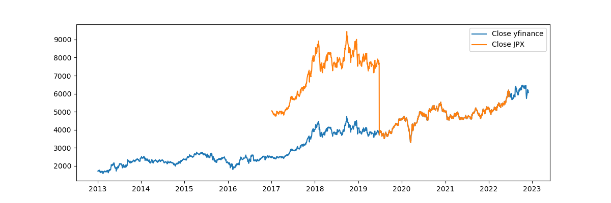
在本文应用
示例代码:
1 | import pandas as pd |
yfinance
yfinance概述
什么是yfinance
Yahoo!finance(雅虎财经),最初有官方的免费的API,但是因为被滥用,官方的API已经于2017年5月15日停止了。
yfinance,是非官方的,数据依旧来自雅虎,但其实是通过类似爬虫的技术实现的。
安装
安装:
1 | pip install yfinance |
在中国大陆使用
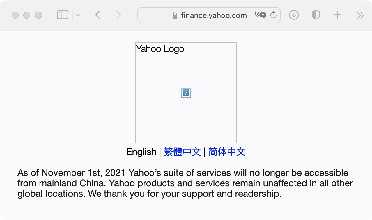
因为从2021年11月1日开始,Yahoo已经不再对中国大陆提供服务。同时,因为yfinance没有代理功能,在中国大陆使用yfinance,可能会收到如下报错
1 | HTTPError: 403 Client Error: Forbidden for url: https://query2.finance.yahoo.com/v10/finance/quoteSummary/600000.SS?modules=summaryProfile%2CfinancialData%2CquoteType%2CdefaultKeyStatistics%2CassetProfile%2CsummaryDetail&ssl=true |
因此,在中国大陆使用,需要自行挂载代理。
如果报了类似如下的错误
error:No timezone found, symbol may be delistederror:No data found for this date range, symbol may be delisted
其原因是被反爬了。
优点
yfinance的优点有:
- 免费
- 无需注册,无需Token
- 数据粒度高(1min/2min/5min数据)
- 直接以Pandas中的
DataFrame或者Series的形式返回数据。
缺点
yfinance的缺点有:
yfinance其实是通过一种类似爬虫的技术从雅虎财经获取数据的,为了避免被反爬,在使用的过程中,还是需要注意。- 在中国大陆使用不方便
模块
yfinance分为三个模块:
Tickersdownloadpandas_datareader
其中,download功能,无法在中国大陆使用(挂载高匿代理或许可以);pandas_datareader,是为了与遗留代码向后兼容。我们只讨论Tickers。
Tickers
info,获取股票基本信息
info,获取股票基本信息。一个股票的基本信息有很多内容。示例代码:
1 | import yfinance as yf |
运行结果:
1 | { |
history,获取历史数据
history,获取历史数据,有以下几个参数可供配置:
period表示获取多久的数据,有10种选择:1d、5d、1mo、3mo、6mo、1y、2y、5y、10y、ytd、max。interval,表示数据的精度,有13种选择:1m、2m、5m、15m、30m、60m、90m、1h、1d、5d、1wk、1mo、3mo。
天以内(不含天)的数据只能最多采集60天以内的,精度越高,能采集的数据天数更少,比如1m数据只能采集7天以内的。start,如果没有配置period,可以使用start(数据开始时间)和end(数据结束时间)来定义应该获取多久的数据。end,同上。prepost,是否包含盘前和盘后价格,默认False不包含auto_adjust,是否自动复权(前复权),默认True。actions,是否包含分红和扩股信息,默认True。
示例代码:
1 | import yfinance as yf |
运行结果:
注意!auto_adjust=False,即不进行复权。但是我们看到,在yfinance中,auto_adjust=False,对于拆股依旧进行了复权,但是对于分红,没有复权。
actions,获取股票的分红和扩股数据
示例代码:
1 | t1414.actions |
运行结果:
1 | Dividends Stock Splits |
dividends,只看股票的分红数据
示例代码:
1 | t1414.dividends |
运行结果:
1 | Date |
splits,只看股票的扩股数据
示例代码:
1 | t1414.splits |
运行结果:
1 | Date |
更多信息
其他更多信息有:
- 获取重要持股人信息:
major_holders - 获取重要机构持股人信息:
institutional_holders - 获取共同基金持股人信息:
mutualfund_holders - 当季财年信息:
calendar - 年度营业收入和税后收益:
earnings - 季度营业收入和税后收益:
quarterly_earnings - 年度详细财报:
financials - 季度详细财报:
quarterly_financials - 年度资产负债表:
balance_sheet - 季度资产负债表:
quarterly_balance_sheet - 年度现金流:
cashflow - 季度现金流:
quarterly_cashflow
在本文的应用
示例代码:
1 | import pandas as pd |
注意!time.sleep(2),这个一定要有,否则会被反爬。