本章会讨论:
分析衍生特征 时序特征衍生 借鉴文本处理 测试集的特征衍生 目标编码
在上一章《特征工程-2.特征衍生 [1/2]》 ,我们讨论了:
根据第一章《特征工程-1.特征预处理》 的讨论,我们对数据进行如下操作,本文的讨论都在此基础上。
示例代码:
1
2
3
4
5
6
7
8
9
10
11
12
13
14
15
16
17
18
19
20
21
22
23
24
25
26
27
28
29
30
31
32
33
34
35
36
37
38
39
40
41
42
43
44
45
46
import pandas as pdimport numpy as nppd.set_option('display.max_columns' , None ) pd.set_option('display.width' , 5000 ) t = pd.read_csv('WA_Fn-UseC_-Telco-Customer-Churn.csv' ) category_cols = ['gender' , 'SeniorCitizen' , 'Partner' , 'Dependents' , 'PhoneService' , 'MultipleLines' , 'InternetService' , 'OnlineSecurity' , 'OnlineBackup' , 'DeviceProtection' , 'TechSupport' , 'StreamingTV' , 'StreamingMovies' , 'Contract' , 'PaperlessBilling' , 'PaymentMethod' ] numeric_cols = ['tenure' , 'MonthlyCharges' , 'TotalCharges' ] target = 'Churn' ID_col = 'customerID' t['TotalCharges' ] = t['TotalCharges' ].apply(lambda x: x if x != ' ' else np.nan).astype(float) t['MonthlyCharges' ] = t['MonthlyCharges' ].astype(float) t['TotalCharges' ] = t['TotalCharges' ].fillna(0 ) t['Churn' ].replace(to_replace='Yes' , value=1 , inplace=True ) t['Churn' ].replace(to_replace='No' , value=0 , inplace=True ) features = t.drop(columns=[ID_col, target]).copy() labels = t['Churn' ].copy() print(features.head(5 )) print('-' * 10 ) print(labels)
运行结果:
1
2
3
4
5
6
7
8
9
10
11
12
13
14
15
16
17
18
19
gender SeniorCitizen Partner Dependents tenure PhoneService MultipleLines InternetService OnlineSecurity OnlineBackup DeviceProtection TechSupport StreamingTV StreamingMovies Contract PaperlessBilling PaymentMethod MonthlyCharges TotalCharges 0 Female 0 Yes No 1 No No phone service DSL No Yes No No No No Month-to-month Yes Electronic check 29.85 29.85 1 Male 0 No No 34 Yes No DSL Yes No Yes No No No One year No Mailed check 56.95 1889.50 2 Male 0 No No 2 Yes No DSL Yes Yes No No No No Month-to-month Yes Mailed check 53.85 108.15 3 Male 0 No No 45 No No phone service DSL Yes No Yes Yes No No One year No Bank transfer (automatic) 42.30 1840.75 4 Female 0 No No 2 Yes No Fiber optic No No No No No No Month-to-month Yes Electronic check 70.70 151.65 ---------- 0 0 1 0 2 1 3 0 4 1 .. 7038 0 7039 0 7040 0 7041 1 7042 0 Name: Churn, Length: 7043, dtype: int64
分析衍生特征
概述
分析衍生特征,也被称为手动衍生特征、人工特征衍生,是指是在经过一定分析后,手动合成一些特征。
整体上,分析衍生特征的思路有两种:
从数据业务出发。
从模型结果出发。
在本文,我们讨论第一种。
标签值分布
查看标签字段的取值分布情况。示例代码:
1 2 print(f'Percentage of Churn: {round(labels.value_counts(normalize=True )[1 ] * 100 , 2 )} % --> ({labels.value_counts()[1 ]} customer)' ) print(f'Percentage of customer did not churn: {round(labels.value_counts(normalize=True )[0 ] * 100 , 2 )} % --> ({labels.value_counts()[0 ]} customer)' )
运行结果:
1
2
Percentage of Churn: 26.54% --> (1869 customer) Percentage of customer did not churn: 73.46% --> (5174 customer)
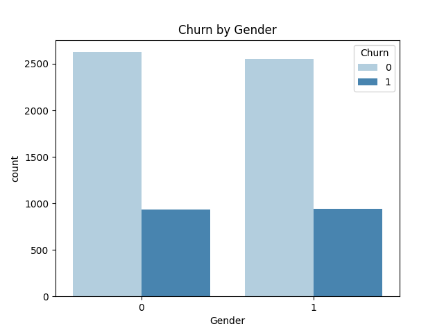
在一共7043条数据中,流失用户占比约为26.54%,整体来看标签取值并不均匀。
我们还可以以其中某一个特征为例,以柱状图的方式,查看其与标签之间的相关性。示例代码:
1 2 3 4 sns.countplot(x="gender_Female" , hue="Churn" , data=df_dummies, palette="Blues" , dodge=True ) plt.xlabel("Gender" ) plt.title("Churn by Gender" ) plt.show()
运行结果:
相关性分析
皮尔逊相关系数
在严格的统计学的框架下,不同类型变量的相关性需要采用不同的分析方法。
连续变量之间的相关性,使用皮尔逊相关系数。
连续变量和离散变量之间的相关性,使用卡方检验。
离散变量之间的相关性,从信息增益角度进行分析。
在本文,我们暂且只是探查特征之间是否存在相关关系,因此忽略连续或离散的特性,统一使用皮尔逊相关系数进行计算。
皮尔逊相关系数的计算公式如下:
r x y = ∑ i = 1 n ( x i − x ˉ ) ( y i − y ˉ ) ∑ i = 1 n ( x i − x ˉ ) 2 ∑ i = 1 n ( y i − y ˉ ) 2 r_{xy}=\frac{\sum_{i=1}^{n}(x_i-\bar{ x})(y_i-\bar{y})}{\sqrt{\sum_{i=1}^{n}(x_i-\bar{ x})^2}\sqrt{\sum_{i=1}^{n}(y_i-\bar{y})^2}}
r x y = ∑ i = 1 n ( x i − x ˉ ) 2 ∑ i = 1 n ( y i − y ˉ ) 2 ∑ i = 1 n ( x i − x ˉ ) ( y i − y ˉ )
r x y r_{xy} r x y x x x y y y n n n x i x_i x i y i y_i y i i i i x ˉ \bar{ x} x ˉ y ˉ \bar{y} y ˉ x x x y y y ∑ i = 1 n \sum_{i=1}^{n} ∑ i = 1 n i = 1 i=1 i = 1 i = n i=n i = n
皮尔逊相关系数,范围是[ − 1 , + 1 ] [-1,+1] [ − 1 , + 1 ] 0 0 0 + 1 +1 + 1 − 1 -1 − 1
pd.get_dummies
首先,我们需要对离散特征进行0-1编码。《特征工程-1.特征预处理》 ,我们讨论过OneHotEncoder。在本文,我们采用另一种方法,pd.get_dummies。
示例代码:
1
2
3
4
5
df_corr = pd.concat([features, labels], axis=1 ) print(df_corr.info()) df_dummies = pd.get_dummies(df_corr) print(df_dummies)
运行结果:
1
2
3
4
5
6
7
8
9
10
11
12
13
14
15
16
17
18
19
20
21
22
23
24
25
26
27
28
29
30
31
32
33
34
35
36
37
38
39
40
41
42
<class 'pandas.core.frame.DataFrame'> RangeIndex: 7043 entries, 0 to 7042 Data columns (total 20 columns): # Column Non-Null Count Dtype --- ------ -------------- ----- 0 gender 7043 non-null object 1 SeniorCitizen 7043 non-null int64 2 Partner 7043 non-null object 3 Dependents 7043 non-null object 4 tenure 7043 non-null int64 5 PhoneService 7043 non-null object 6 MultipleLines 7043 non-null object 7 InternetService 7043 non-null object 8 OnlineSecurity 7043 non-null object 9 OnlineBackup 7043 non-null object 10 DeviceProtection 7043 non-null object 11 TechSupport 7043 non-null object 12 StreamingTV 7043 non-null object 13 StreamingMovies 7043 non-null object 14 Contract 7043 non-null object 15 PaperlessBilling 7043 non-null object 16 PaymentMethod 7043 non-null object 17 MonthlyCharges 7043 non-null float64 18 TotalCharges 7043 non-null float64 19 Churn 7043 non-null int64 dtypes: float64(2), int64(3), object(15) memory usage: 1.1+ MB None SeniorCitizen tenure MonthlyCharges TotalCharges Churn gender_Female gender_Male Partner_No Partner_Yes Dependents_No Dependents_Yes PhoneService_No PhoneService_Yes MultipleLines_No MultipleLines_No phone service MultipleLines_Yes InternetService_DSL InternetService_Fiber optic InternetService_No OnlineSecurity_No OnlineSecurity_No internet service OnlineSecurity_Yes OnlineBackup_No OnlineBackup_No internet service OnlineBackup_Yes DeviceProtection_No DeviceProtection_No internet service DeviceProtection_Yes TechSupport_No TechSupport_No internet service TechSupport_Yes StreamingTV_No StreamingTV_No internet service StreamingTV_Yes StreamingMovies_No StreamingMovies_No internet service StreamingMovies_Yes Contract_Month-to-month Contract_One year Contract_Two year PaperlessBilling_No PaperlessBilling_Yes PaymentMethod_Bank transfer (automatic) PaymentMethod_Credit card (automatic) PaymentMethod_Electronic check PaymentMethod_Mailed check 0 0 1 29.85 29.85 0 1 0 0 1 1 0 1 0 0 1 0 1 0 0 1 0 0 0 0 1 1 0 0 1 0 0 1 0 0 1 0 0 1 0 0 0 1 0 0 1 0 1 0 34 56.95 1889.50 0 0 1 1 0 1 0 0 1 1 0 0 1 0 0 0 0 1 1 0 0 0 0 1 1 0 0 1 0 0 1 0 0 0 1 0 1 0 0 0 0 1 2 0 2 53.85 108.15 1 0 1 1 0 1 0 0 1 1 0 0 1 0 0 0 0 1 0 0 1 1 0 0 1 0 0 1 0 0 1 0 0 1 0 0 0 1 0 0 0 1 3 0 45 42.30 1840.75 0 0 1 1 0 1 0 1 0 0 1 0 1 0 0 0 0 1 1 0 0 0 0 1 0 0 1 1 0 0 1 0 0 0 1 0 1 0 1 0 0 0 4 0 2 70.70 151.65 1 1 0 1 0 1 0 0 1 1 0 0 0 1 0 1 0 0 1 0 0 1 0 0 1 0 0 1 0 0 1 0 0 1 0 0 0 1 0 0 1 0 ... ... ... ... ... ... ... ... ... ... ... ... ... ... ... ... ... ... ... ... ... ... ... ... ... ... ... ... ... ... ... ... ... ... ... ... ... ... ... ... ... ... ... ... ... ... ... 7038 0 24 84.80 1990.50 0 0 1 0 1 0 1 0 1 0 0 1 1 0 0 0 0 1 1 0 0 0 0 1 0 0 1 0 0 1 0 0 1 0 1 0 0 1 0 0 0 1 7039 0 72 103.20 7362.90 0 1 0 0 1 0 1 0 1 0 0 1 0 1 0 1 0 0 0 0 1 0 0 1 1 0 0 0 0 1 0 0 1 0 1 0 0 1 0 1 0 0 7040 0 11 29.60 346.45 0 1 0 0 1 0 1 1 0 0 1 0 1 0 0 0 0 1 1 0 0 1 0 0 1 0 0 1 0 0 1 0 0 1 0 0 0 1 0 0 1 0 7041 1 4 74.40 306.60 1 0 1 0 1 1 0 0 1 0 0 1 0 1 0 1 0 0 1 0 0 1 0 0 1 0 0 1 0 0 1 0 0 1 0 0 0 1 0 0 0 1 7042 0 66 105.65 6844.50 0 0 1 1 0 1 0 0 1 1 0 0 0 1 0 0 0 1 1 0 0 0 0 1 0 0 1 0 0 1 0 0 1 0 0 1 0 1 1 0 0 0 [7043 rows x 46 columns]
在上文,我们有意打印了df_corr.info(),可以看到,pd.get_dummies会将非数值类型对象类型进行自动哑变量转化,对于数值类型对象,无论是整型还是浮点型,都会保留原始列不变。
corr()计算相关系数矩阵
利用corr()计算相关系数矩阵。示例代码:
1 print(df_dummies.corr())
运行结果:
1
2
3
4
5
6
7
8
9
10
11
12
13
14
SeniorCitizen tenure MonthlyCharges TotalCharges Churn gender_Female gender_Male Partner_No Partner_Yes Dependents_No Dependents_Yes PhoneService_No PhoneService_Yes MultipleLines_No MultipleLines_No phone service MultipleLines_Yes InternetService_DSL InternetService_Fiber optic InternetService_No OnlineSecurity_No OnlineSecurity_No internet service OnlineSecurity_Yes OnlineBackup_No OnlineBackup_No internet service OnlineBackup_Yes DeviceProtection_No DeviceProtection_No internet service DeviceProtection_Yes TechSupport_No TechSupport_No internet service TechSupport_Yes StreamingTV_No StreamingTV_No internet service StreamingTV_Yes StreamingMovies_No StreamingMovies_No internet service StreamingMovies_Yes Contract_Month-to-month Contract_One year Contract_Two year PaperlessBilling_No PaperlessBilling_Yes PaymentMethod_Bank transfer (automatic) PaymentMethod_Credit card (automatic) PaymentMethod_Electronic check PaymentMethod_Mailed check SeniorCitizen 1.000000 0.016567 0.220173 0.103006 0.150889 0.001874 -0.001874 -0.016479 0.016479 0.211185 -0.211185 -0.008576 0.008576 -0.136213 -0.008576 0.142948 -0.108322 0.255338 -0.182742 0.185532 -0.182742 -0.038653 0.087952 -0.182742 0.066572 0.094810 -0.182742 0.059428 0.205620 -0.182742 -0.060625 0.049062 -0.182742 0.105378 0.034210 -0.182742 0.120176 0.138360 -0.046262 -0.117000 -0.156530 0.156530 -0.016159 -0.024135 0.171718 -0.153477 tenure 0.016567 1.000000 0.247900 0.826178 -0.352229 -0.005106 0.005106 -0.379697 0.379697 -0.159712 0.159712 -0.008448 0.008448 -0.323088 -0.008448 0.331941 0.013274 0.019720 -0.039062 -0.263746 -0.039062 0.327203 -0.312694 -0.039062 0.360277 -0.312740 -0.039062 0.360653 -0.262143 -0.039062 0.324221 -0.245039 -0.039062 0.279756 -0.252220 -0.039062 0.286111 -0.645561 0.202570 0.558533 -0.006152 0.006152 0.243510 0.233006 -0.208363 -0.233852 MonthlyCharges 0.220173 0.247900 1.000000 0.651174 0.193356 0.014569 -0.014569 -0.096848 0.096848 0.113890 -0.113890 -0.247398 0.247398 -0.338314 -0.247398 0.490434 -0.160189 0.787066 -0.763557 0.360898 -0.763557 0.296594 0.210753 -0.763557 0.441780 0.171836 -0.763557 0.482692 0.322076 -0.763557 0.338304 0.016951 -0.763557 0.629603 0.018075 -0.763557 0.627429 0.060165 0.004904 -0.074681 -0.352150 0.352150 0.042812 0.030550 0.271625 -0.377437 TotalCharges 0.103006 0.826178 0.651174 1.000000 -0.198324 0.000080 -0.000080 -0.317504 0.317504 -0.062078 0.062078 -0.113214 0.113214 -0.396059 -0.113214 0.468504 -0.052469 0.361655 -0.375223 -0.063137 -0.375223 0.411651 -0.176276 -0.375223 0.509226 -0.188108 -0.375223 0.521983 -0.082874 -0.375223 0.431883 -0.195884 -0.375223 0.514973 -0.202188 -0.375223 0.520122 -0.444255 0.170814 0.354481 -0.158574 0.158574 0.185987 0.182915 -0.059246 -0.295758 Churn 0.150889 -0.352229 0.193356 -0.198324 1.000000 0.008612 -0.008612 0.150448 -0.150448 0.164221 -0.164221 -0.011942 0.011942 -0.032569 -0.011942 0.040102 -0.124214 0.308020 -0.227890 0.342637 -0.227890 -0.171226 0.268005 -0.227890 -0.082255 0.252481 -0.227890 -0.066160 0.337281 -0.227890 -0.164674 0.128916 -0.227890 0.063228 0.130845 -0.227890 0.061382 0.405103 -0.177820 -0.302253 -0.191825 0.191825 -0.117937 -0.134302 0.301919 -0.091683 【部分运行结果略】 PaperlessBilling_Yes 0.156530 0.006152 0.352150 0.158574 0.191825 0.011754 -0.011754 0.014877 -0.014877 0.111377 -0.111377 -0.016505 0.016505 -0.151864 -0.016505 0.163530 -0.063121 0.326853 -0.321013 0.267793 -0.321013 -0.003636 0.145120 -0.321013 0.126735 0.167121 -0.321013 0.103797 0.230136 -0.321013 0.037880 0.047712 -0.321013 0.223841 0.059488 -0.321013 0.211716 0.169096 -0.051391 -0.147889 -1.000000 1.000000 -0.016332 -0.013589 0.208865 -0.205398 PaymentMethod_Bank transfer (automatic) -0.016159 0.243510 0.042812 0.185987 -0.117937 0.016024 -0.016024 -0.110706 0.110706 -0.052021 0.052021 -0.007556 0.007556 -0.070178 -0.007556 0.075527 0.025476 -0.022624 -0.002113 -0.084322 -0.002113 0.095158 -0.081590 -0.002113 0.087004 -0.077791 -0.002113 0.083115 -0.090177 -0.002113 0.101252 -0.044168 -0.002113 0.046252 -0.046705 -0.002113 0.048652 -0.179707 0.057451 0.154471 0.016332 -0.016332 1.000000 -0.278215 -0.376762 -0.288685 PaymentMethod_Credit card (automatic) -0.024135 0.233006 0.030550 0.182915 -0.134302 -0.001215 0.001215 -0.082029 0.082029 -0.060267 0.060267 0.007721 -0.007721 -0.063921 0.007721 0.060048 0.051438 -0.050077 0.001030 -0.105510 0.001030 0.115721 -0.087822 0.001030 0.090785 -0.107618 0.001030 0.111554 -0.107310 0.001030 0.117272 -0.041031 0.001030 0.040433 -0.049277 0.001030 0.048575 -0.204145 0.067589 0.173265 0.013589 -0.013589 -0.278215 1.000000 -0.373322 -0.286049 PaymentMethod_Electronic check 0.171718 -0.208363 0.271625 -0.059246 0.301919 -0.000752 0.000752 0.083852 -0.083852 0.150642 -0.150642 -0.003062 0.003062 -0.080836 -0.003062 0.083618 -0.104418 0.336410 -0.284917 0.336364 -0.284917 -0.112338 0.236947 -0.284917 -0.000408 0.239705 -0.284917 -0.003351 0.339031 -0.284917 -0.114839 0.096033 -0.284917 0.144626 0.102571 -0.284917 0.137966 0.331661 -0.109130 -0.282138 -0.208865 0.208865 -0.376762 -0.373322 1.000000 -0.387372 PaymentMethod_Mailed check -0.153477 -0.233852 -0.377437 -0.295758 -0.091683 -0.013744 0.013744 0.095125 -0.095125 -0.059071 0.059071 0.003319 -0.003319 0.222605 0.003319 -0.227206 0.041899 -0.306834 0.321361 -0.191715 0.321361 -0.080798 -0.099975 0.321361 -0.174164 -0.087422 0.321361 -0.187373 -0.187185 0.321361 -0.085509 -0.024261 0.321361 -0.247742 -0.021034 0.321361 -0.250595 0.004138 -0.000116 -0.004705 0.205398 -0.205398 -0.288685 -0.286049 -0.387372 1.000000
df_dummies.corr()的运算结果就是一个DataFrame。示例代码:
1 print(type(df_dummies.corr()))
运行结果:
1 <class 'pandas.core.frame.DataFrame'>
我们重点关注特征和标签之间的相关性。示例代码:
1 print(df_dummies.corr()['Churn' ].sort_values(ascending=False ))
运行结果:
1
2
3
4
5
6
7
8
9
10
11
12
13
14
15
16
17
18
19
20
21
22
23
24
25
26
27
28
29
30
31
32
33
34
35
36
37
38
39
40
41
42
43
44
45
46
47
Churn 1.000000 Contract_Month-to-month 0.405103 OnlineSecurity_No 0.342637 TechSupport_No 0.337281 InternetService_Fiber optic 0.308020 PaymentMethod_Electronic check 0.301919 OnlineBackup_No 0.268005 DeviceProtection_No 0.252481 MonthlyCharges 0.193356 PaperlessBilling_Yes 0.191825 Dependents_No 0.164221 SeniorCitizen 0.150889 Partner_No 0.150448 StreamingMovies_No 0.130845 StreamingTV_No 0.128916 StreamingTV_Yes 0.063228 StreamingMovies_Yes 0.061382 MultipleLines_Yes 0.040102 PhoneService_Yes 0.011942 gender_Female 0.008612 gender_Male -0.008612 MultipleLines_No phone service -0.011942 PhoneService_No -0.011942 MultipleLines_No -0.032569 DeviceProtection_Yes -0.066160 OnlineBackup_Yes -0.082255 PaymentMethod_Mailed check -0.091683 PaymentMethod_Bank transfer (automatic) -0.117937 InternetService_DSL -0.124214 PaymentMethod_Credit card (automatic) -0.134302 Partner_Yes -0.150448 Dependents_Yes -0.164221 TechSupport_Yes -0.164674 OnlineSecurity_Yes -0.171226 Contract_One year -0.177820 PaperlessBilling_No -0.191825 TotalCharges -0.198324 DeviceProtection_No internet service -0.227890 StreamingMovies_No internet service -0.227890 InternetService_No -0.227890 OnlineSecurity_No internet service -0.227890 StreamingTV_No internet service -0.227890 TechSupport_No internet service -0.227890 OnlineBackup_No internet service -0.227890 Contract_Two year -0.302253 tenure -0.352229 Name: Churn, dtype: float64
绘图展示
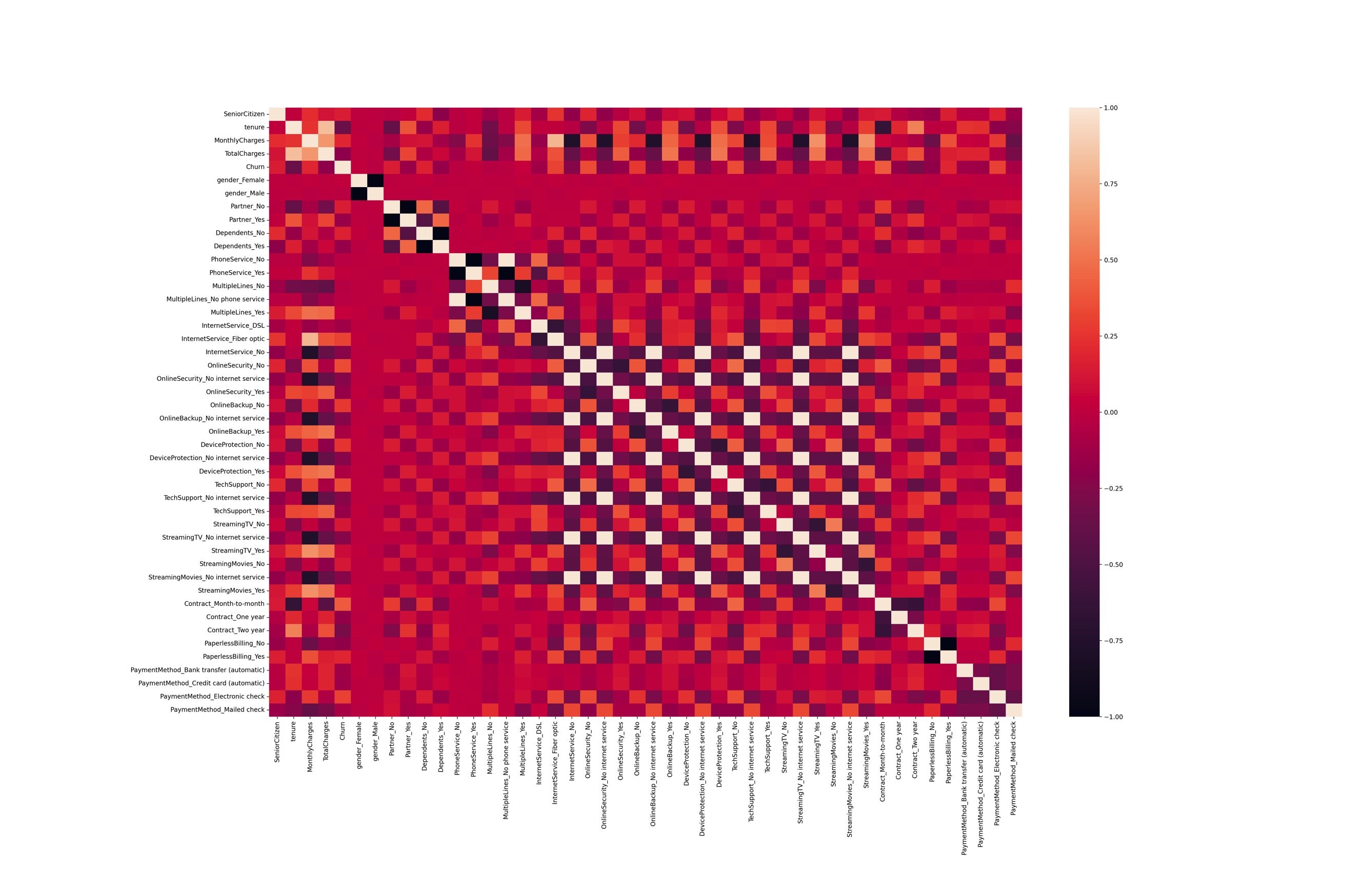
热力图展示相关性
示例代码:
1
2
3
4
5
6
7
8
import matplotlib.pyplot as pltimport seaborn as snsplt.figure(figsize=(30 , 20 ), dpi=200 ) plt.subplots_adjust(bottom=0.2 ) plt.subplots_adjust(left=0.2 ) sns.heatmap(df_dummies.corr()) plt.show()
运行结果:
解释说明:.subplots_adjust(bottom=0.2)和.subplots_adjust(left=0.2)分别调整了图的底部和左侧边缘的位置,使得图中文字或坐标值不会被边框覆盖或过于拥挤。如果不进行调整,因为图的边缘位置可能会被默认值挡住一部分,给观察和分析带来一定困难。
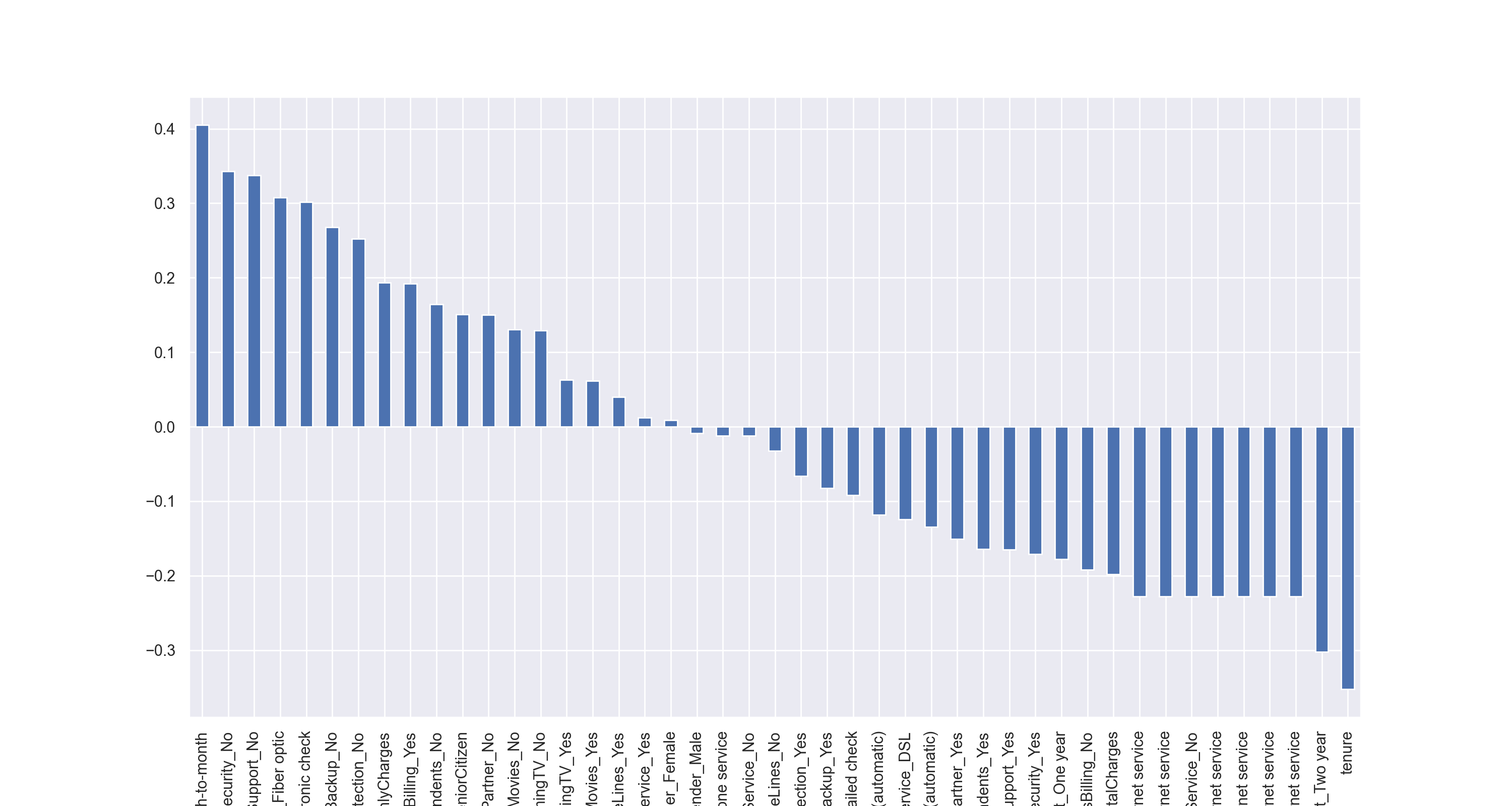
柱状图展示相关性
对于具体某一个特征和其他特征的相关性,热力图的展示结果并不直观,此时我们可以考虑使用柱状图来展示。
示例代码:
1
2
3
4
5
6
7
import matplotlib.pyplot as pltimport seaborn as snssns.set() plt.figure(figsize=(15 , 8 ), dpi=200 ) df_dummies.corr()['Churn' ].sort_values(ascending=False )[1 :].plot(kind='bar' ) plt.show()
运行结果:
解释说明:上述代码的[1:],作用是去除相关性最大的一个。根据上文,我们知道和Churn的相关性最大的是Churn本身。
衍生新特征
思路
上文我们对数据进行了一定的分析。
新用户标识
购买服务指数
现在,我们来手动合成这两个特征。
新用户标识
标识规则
tenure表示的是用户入网时间,如果用户的tenure小于某个值,我就认为是新用户。
首先查看tenure的所有取值,示例代码:
1 print(np.sort(df_dummies['tenure' ].unique()))
运行结果:
1
2
3
4
[ 0 1 2 3 4 5 6 7 8 9 10 11 12 13 14 15 16 17 18 19 20 21 22 23 24 25 26 27 28 29 30 31 32 33 34 35 36 37 38 39 40 41 42 43 44 45 46 47 48 49 50 51 52 53 54 55 56 57 58 59 60 61 62 63 64 65 66 67 68 69 70 71 72]
现在,假定,我们将所有tenure取值为0或1的用户标识为新用户,据此衍生出一个二分类(0/1,1表示新用户)的特征,new_customer。
新特征的生成
示例代码:
1 2 3 4 5 6 new_customer_con = (features['tenure' ] <= 1 ) print(new_customer_con) new_customer = (new_customer_con * 1 ).values print(new_customer)
运行结果:
1
2
3
4
5
6
7
8
9
10
11
12
13
0 True 1 False 2 False 3 False 4 False ... 7038 False 7039 False 7040 False 7041 False 7042 False Name: tenure, Length: 7043, dtype: bool [1 0 0 ... 0 0 0]
新特征的组装
示例代码:
1
2
3
print(features) features['new_customer' ] = new_customer print(features)
运行结果:
1
2
3
4
5
6
7
8
9
10
11
12
13
14
15
16
17
18
19
20
21
22
23
24
25
26
27
28
gender SeniorCitizen Partner Dependents tenure PhoneService MultipleLines InternetService OnlineSecurity OnlineBackup DeviceProtection TechSupport StreamingTV StreamingMovies Contract PaperlessBilling PaymentMethod MonthlyCharges TotalCharges 0 Female 0 Yes No 1 No No phone service DSL No Yes No No No No Month-to-month Yes Electronic check 29.85 29.85 1 Male 0 No No 34 Yes No DSL Yes No Yes No No No One year No Mailed check 56.95 1889.50 2 Male 0 No No 2 Yes No DSL Yes Yes No No No No Month-to-month Yes Mailed check 53.85 108.15 3 Male 0 No No 45 No No phone service DSL Yes No Yes Yes No No One year No Bank transfer (automatic) 42.30 1840.75 4 Female 0 No No 2 Yes No Fiber optic No No No No No No Month-to-month Yes Electronic check 70.70 151.65 ... ... ... ... ... ... ... ... ... ... ... ... ... ... ... ... ... ... ... ... 7038 Male 0 Yes Yes 24 Yes Yes DSL Yes No Yes Yes Yes Yes One year Yes Mailed check 84.80 1990.50 7039 Female 0 Yes Yes 72 Yes Yes Fiber optic No Yes Yes No Yes Yes One year Yes Credit card (automatic) 103.20 7362.90 7040 Female 0 Yes Yes 11 No No phone service DSL Yes No No No No No Month-to-month Yes Electronic check 29.60 346.45 7041 Male 1 Yes No 4 Yes Yes Fiber optic No No No No No No Month-to-month Yes Mailed check 74.40 306.60 7042 Male 0 No No 66 Yes No Fiber optic Yes No Yes Yes Yes Yes Two year Yes Bank transfer (automatic) 105.65 6844.50 [7043 rows x 19 columns] gender SeniorCitizen Partner Dependents tenure PhoneService MultipleLines InternetService OnlineSecurity OnlineBackup DeviceProtection TechSupport StreamingTV StreamingMovies Contract PaperlessBilling PaymentMethod MonthlyCharges TotalCharges new_customer 0 Female 0 Yes No 1 No No phone service DSL No Yes No No No No Month-to-month Yes Electronic check 29.85 29.85 1 1 Male 0 No No 34 Yes No DSL Yes No Yes No No No One year No Mailed check 56.95 1889.50 0 2 Male 0 No No 2 Yes No DSL Yes Yes No No No No Month-to-month Yes Mailed check 53.85 108.15 0 3 Male 0 No No 45 No No phone service DSL Yes No Yes Yes No No One year No Bank transfer (automatic) 42.30 1840.75 0 4 Female 0 No No 2 Yes No Fiber optic No No No No No No Month-to-month Yes Electronic check 70.70 151.65 0 ... ... ... ... ... ... ... ... ... ... ... ... ... ... ... ... ... ... ... ... ... 7038 Male 0 Yes Yes 24 Yes Yes DSL Yes No Yes Yes Yes Yes One year Yes Mailed check 84.80 1990.50 0 7039 Female 0 Yes Yes 72 Yes Yes Fiber optic No Yes Yes No Yes Yes One year Yes Credit card (automatic) 103.20 7362.90 0 7040 Female 0 Yes Yes 11 No No phone service DSL Yes No No No No No Month-to-month Yes Electronic check 29.60 346.45 0 7041 Male 1 Yes No 4 Yes Yes Fiber optic No No No No No No Month-to-month Yes Mailed check 74.40 306.60 0 7042 Male 0 No No 66 Yes No Fiber optic Yes No Yes Yes Yes Yes Two year Yes Bank transfer (automatic) 105.65 6844.50 0 [7043 rows x 20 columns]
购买服务数量
在本文中,总有九项服务,我们通过如下方式的统计每位用户总共购买的服务数量。示例代码:
1
2
3
4
5
6
7
8
9
10
11
12
13
14
15
service_num = ((features['PhoneService' ] == 'Yes' ) * 1 + (features['MultipleLines' ] == 'Yes' ) * 1 + (features['InternetService' ] == 'Yes' ) * 1 + (features['OnlineSecurity' ] == 'Yes' ) * 1 + (features['OnlineBackup' ] == 'Yes' ) * 1 + (features['DeviceProtection' ] == 'Yes' ) * 1 + (features['TechSupport' ] == 'Yes' ) * 1 + (features['StreamingTV' ] == 'Yes' ) * 1 + (features['StreamingMovies' ] == 'Yes' ) * 1 ).values print(service_num) features['service_num' ] = service_num print(features)
运行结果:
1
2
3
4
5
6
7
8
9
10
11
12
13
14
15
[1 3 3 ... 1 2 6] gender SeniorCitizen Partner Dependents tenure PhoneService MultipleLines InternetService OnlineSecurity OnlineBackup DeviceProtection TechSupport StreamingTV StreamingMovies Contract PaperlessBilling PaymentMethod MonthlyCharges TotalCharges new_customer service_num 0 Female 0 Yes No 1 No No phone service DSL No Yes No No No No Month-to-month Yes Electronic check 29.85 29.85 1 1 1 Male 0 No No 34 Yes No DSL Yes No Yes No No No One year No Mailed check 56.95 1889.50 0 3 2 Male 0 No No 2 Yes No DSL Yes Yes No No No No Month-to-month Yes Mailed check 53.85 108.15 0 3 3 Male 0 No No 45 No No phone service DSL Yes No Yes Yes No No One year No Bank transfer (automatic) 42.30 1840.75 0 3 4 Female 0 No No 2 Yes No Fiber optic No No No No No No Month-to-month Yes Electronic check 70.70 151.65 0 1 ... ... ... ... ... ... ... ... ... ... ... ... ... ... ... ... ... ... ... ... ... ... 7038 Male 0 Yes Yes 24 Yes Yes DSL Yes No Yes Yes Yes Yes One year Yes Mailed check 84.80 1990.50 0 7 7039 Female 0 Yes Yes 72 Yes Yes Fiber optic No Yes Yes No Yes Yes One year Yes Credit card (automatic) 103.20 7362.90 0 6 7040 Female 0 Yes Yes 11 No No phone service DSL Yes No No No No No Month-to-month Yes Electronic check 29.60 346.45 0 1 7041 Male 1 Yes No 4 Yes Yes Fiber optic No No No No No No Month-to-month Yes Mailed check 74.40 306.60 0 2 7042 Male 0 No No 66 Yes No Fiber optic Yes No Yes Yes Yes Yes Two year Yes Bank transfer (automatic) 105.65 6844.50 0 6 [7043 rows x 21 columns]
在实践中,我们可以定义"服务购买指数",比如某些服务比较重要,我们对其乘以5。
1 (features['InternetService' ] == 'Yes' ) * 5
时序特征衍生
概述
时序特征,记录了时间的特征。
但其不仅仅是一个时间格式的字符串,其背后可能隐藏着非常多极有价值的信息(例如,季节性的波动规律)。
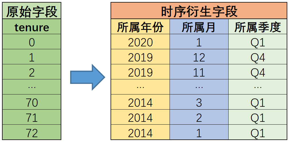
有序数字
衍生过程
根据上文的讨论,tenure入网时间,以月跨度,tenure的取值范围[0, 72]表示过去72个月的时间记录结果,取值越大代表时间越远。tenure=0表示的是2020年1月,tenure=1则代表2019年12月,tenure=2代表2019年11月,依此类推。
现在,我们可以根据tenure衍生出更细粒度的时间信息特征。
实现方法
大小颠倒
为了计算方便(用求余的方式,计算对应的月份的数值),我们对tenure进行大小颠倒,数值越小代表时间越远。即tenure=0表示第一个月、2014年1月,tenure=72表示最后一个月,2020年1月。
示例代码:
1 2 3 print(features['tenure' ].head()) features['tenure' ] = (72 - features['tenure' ]) print(features['tenure' ].head())
运行结果:
1
2
3
4
5
6
7
8
9
10
11
12
0 1 1 34 2 2 3 45 4 2 Name: tenure, dtype: int64 0 71 1 38 2 70 3 27 4 70 Name: tenure, dtype: int64
月份
示例代码:
1 2 features['tenure_month' ] = features['tenure' ] % 12 + 1 print(features[['tenure' , 'tenure_month' ]])
运行结果:
1
2
3
4
5
6
7
8
9
10
11
12
13
14
tenure tenure_month 0 71 2 1 38 11 2 70 3 3 27 10 4 70 3 ... ... ... 7038 48 1 7039 0 1 7040 61 12 7041 68 5 7042 6 7 [7043 rows x 2 columns]
解释说明:月份的值域[ 1 , 12 ] [1,12] [ 1 , 1 2 ] 12 12 1 2 [ 0 , 11 ] [0,11] [ 0 , 1 1 ] + 1 +1 + 1
季度
示例代码:
1 2 features['tenure_quarter' ] = (features['tenure' ] % 12 // 3 ) + 1 print(features[['tenure' , 'tenure_quarter' ]])
运行结果:
1
2
3
4
5
6
7
8
9
10
11
12
13
14
tenure tenure_quarter 0 71 4 1 38 1 2 70 4 3 27 2 4 70 4 ... ... ... 7038 48 1 7039 0 1 7040 61 1 7041 68 3 7042 6 3 [7043 rows x 2 columns]
解释说明:features['tenure'] % 12的值域为[ 0 , 11 ] [0,11] [ 0 , 1 1 ] //的意思为做除法,然后向下取整,之后再+1,即值域是[ 1 , 4 ] [1,4] [ 1 , 4 ]
年份
示例代码:
1 2 features['tenure_year' ] = (features['tenure' ] // 12 ) + 2014 print(features[['tenure' , 'tenure_year' ]])
运行结果:
1
2
3
4
5
6
7
8
9
10
11
12
13
14
tenure tenure_year 0 71 2019 1 38 2017 2 70 2019 3 27 2016 4 70 2019 ... ... ... 7038 48 2018 7039 0 2014 7040 61 2019 7041 68 2019 7042 6 2014 [7043 rows x 2 columns]
解释说明:features['tenure'] % 12的结果为[ 0 , 11 ] [0,11] [ 0 , 1 1 ] //的意思为做除法,然后向下取整,之后再+ 2014 +2014 + 2 0 1 4
相关性分析
我们可以进一步分析用户流失是否和入网年份、月份和季度有关。
示例代码:
1
2
corr_df = pd.concat([features[['tenure_month' , 'tenure_quarter' , 'tenure_year' ]], labels], axis=1 ) print(corr_df.corr())
运行结果:
1
2
3
4
5
tenure_month tenure_quarter tenure_year Churn tenure_month 1.000000 0.975681 0.287452 0.214367 tenure_quarter 0.975681 1.000000 0.269392 0.198723 tenure_year 0.287452 0.269392 1.000000 0.337954 Churn 0.214367 0.198723 0.337954 1.000000
我们还可以将年、月、季度等字段进行One-Hot编码,这样可以看出,具体某一年,某一月和客户流失之间的相关性。
这个步骤,其实隐含了一个思路,我们不再把年月等看作连续特征,即我们的思考角度不是年份每变化一个单位,用户流失的概率相应变化多少。现在我们把年月等看做离散特征了。
示例代码:
1
2
3
4
5
6
7
8
9
10
11
12
col_names = ['tenure_year' , 'tenure_month' , 'tenure_quarter' ] features_t = features[col_names] enc = OneHotEncoder() enc.fit(features_t) features_t = pd.DataFrame(enc.transform(features_t).toarray(), columns=cate_col_name(enc, col_names, skip_binary=True )) features_t['Churn' ] = labels print(abs(features_t.corr()['Churn' ]).sort_values(ascending=False ))
运行结果:
1
2
3
4
5
6
7
8
9
10
11
12
13
14
15
16
17
18
19
20
21
22
23
24
25
Churn 1.000000 tenure_year_2019 0.320054 tenure_month_12 0.194221 tenure_quarter_4 0.184320 tenure_month_11 0.038805 tenure_month_10 0.023090 tenure_year_2018 0.020308 tenure_month_8 0.008940 tenure_month_9 0.006660 tenure_quarter_3 -0.000203 tenure_month_6 -0.014609 tenure_month_7 -0.016201 tenure_year_2020 -0.023771 tenure_month_3 -0.027905 tenure_month_4 -0.032217 tenure_month_5 -0.034115 tenure_year_2017 -0.040637 tenure_quarter_2 -0.050526 tenure_year_2016 -0.059229 tenure_month_2 -0.075770 tenure_year_2015 -0.100416 tenure_month_1 -0.116592 tenure_quarter_1 -0.145929 tenure_year_2014 -0.225500 Name: Churn, dtype: float64
通过分析,我们能看出,2019年入网用户普遍流失率更大,12月和第4季度入网用户普遍容易流失。
特别的,我们可以先求绝对值,然后根据绝对值进行排序。这样找相关性较大的(正相关和负相关,都认为是相关性大)。
1 print(abs(features_t.corr()['Churn' ]).sort_values(ascending=False ))
运行结果:
1
2
3
4
5
6
7
8
9
10
11
12
13
14
15
16
17
18
19
20
21
22
23
24
25
Churn 1.000000 tenure_year_2019 0.320054 tenure_year_2014 0.225500 tenure_month_12 0.194221 tenure_quarter_4 0.184320 tenure_quarter_1 0.145929 tenure_month_1 0.116592 tenure_year_2015 0.100416 tenure_month_2 0.075770 tenure_year_2016 0.059229 tenure_quarter_2 0.050526 tenure_year_2017 0.040637 tenure_month_11 0.038805 tenure_month_5 0.034115 tenure_month_4 0.032217 tenure_month_3 0.027905 tenure_year_2020 0.023771 tenure_month_10 0.023090 tenure_year_2018 0.020308 tenure_month_7 0.016201 tenure_month_6 0.014609 tenure_month_8 0.008940 tenure_month_9 0.006660 tenure_quarter_3 0.000203 Name: Churn, dtype: float64
我们可以进一步分析,是某一年的12月客户流失率较大,还是普遍的12月份客户流失率较大。
示例代码:
1
2
3
4
5
6
7
8
9
10
11
12
13
14
15
16
17
18
19
20
col_names = ['tenure' ] features_t = features[col_names] features_t = features_t.copy() features_t['Churn' ] = labels features_t = features_t[features_t['tenure' ] % 12 == 11 ] features_t_label = features_t['Churn' ] features_t = features_t[['tenure' ]] enc = OneHotEncoder() enc.fit(features_t) features_t = pd.DataFrame(enc.transform(features_t).toarray(), columns=cate_col_name(enc, col_names, skip_binary=True )) features_t['Churn' ] = features_t_label print(features_t.corr()['Churn' ].sort_values(ascending=False ))
运行结果:
1
2
3
4
5
6
7
8
Churn 1.000000 tenure_59 0.158281 tenure_11 0.093483 tenure_23 -0.011704 tenure_47 -0.038867 tenure_35 -0.072028 tenure_71 -0.095818 Name: Churn, dtype: float64
解释说明:第59个月入网的用户,显然更容易流失。
时间格式
时间差值衍生
计算方法
两列相减
示例代码:
1
2
3
4
5
6
7
8
9
10
11
import pandas as pdt = pd.DataFrame() t['time' ] = ['2022-01-03 02:31:52' , '2022-07-01 14:22:01' , '2022-08-22 08:02:31' , '2022-04-30 11:41:31' , '2022-05-02 22:01:27' ] t['time' ] = pd.to_datetime(t['time' ]) print(t['time' ] - t['time' ])
运行结果:
1
2
3
4
5
6
0 0 days 1 0 days 2 0 days 3 0 days 4 0 days Name: time, dtype: timedelta64[ns]
减去指定时间
定义指定时间的方法有两种:
pd.Timestamppd.to_datetime
示例代码:
1
2
3
4
t1 = '2022-01-03 02:31:52' print(t['time' ] - pd.Timestamp(t1)) print(t['time' ] - pd.to_datetime(t1))
运行结果:
1
2
3
4
5
6
7
8
9
10
11
12
0 0 days 00:00:00 1 179 days 11:50:09 2 231 days 05:30:39 3 117 days 09:09:39 4 119 days 19:29:35 Name: time, dtype: timedelta64[ns] 0 0 days 00:00:00 1 179 days 11:50:09 2 231 days 05:30:39 3 117 days 09:09:39 4 119 days 19:29:35 Name: time, dtype: timedelta64[ns]
天数
从计算结果中,提取天数,td.dt.days。
示例代码:
1
2
3
td = t['time' ] - pd.to_datetime(t1) print(td.dt.days)
运行结果:
1
2
3
4
5
6
0 0 1 179 2 231 3 117 4 119 Name: time, dtype: int64
解释说明:相差的天数是完全忽略时分秒的结果。
秒数
忽略了天数的计算结果
从计算结果中,提取秒数,td.dt.seconds。
示例代码:
1
2
3
td = t['time' ] - pd.to_datetime(t1) print(td.dt.seconds)
运行结果:
1
2
3
4
5
6
0 0 1 42609 2 19839 3 32979 4 70175 Name: time, dtype: int64
解释说明:相差的秒数则是完全忽略了天数的计算结果
获取所有的秒数
那么,如果我们想计算时间差的所有秒数呢?24 ∗ 60 ∗ 60 24*60*60 2 4 ∗ 6 0 ∗ 6 0
关于Numpy中的时间处理,可以参考《2.numpy》 。
小时数:td.values.astype('timedelta64[h]')td.values.astype('timedelta64[s]')
示例代码:
1 2 print(td.values.astype('timedelta64[h]' )) print(td.values.astype('timedelta64[s]' ))
运行结果:
1
2
[ 0 4307 5549 2817 2875] [ 0 15508209 19978239 10141779 10351775]
好!已经获取成功了!现在我们再把特征组装回去。示例代码:
1
2
3
4
5
6
7
8
9
10
11
12
13
14
15
16
17
18
19
import pandas as pdt = pd.DataFrame() t['time' ] = ['2022-01-03 02:31:52' , '2022-07-01 14:22:01' , '2022-08-22 08:02:31' , '2022-04-30 11:41:31' , '2022-05-02 22:01:27' ] t['time' ] = pd.to_datetime(t['time' ]) t1 = '2022-01-03 02:31:52' td = (t['time' ] - pd.to_datetime(t1)).values.astype('timedelta64[s]' ) print(td) t['tdiff_s' ] = td print(t['tdiff_s' ].dt.seconds)
运行结果:
1
2
3
4
5
6
7
[ 0 15508209 19978239 10141779 10351775] 0 0 1 42609 2 19839 3 32979 4 70175 Name: tdiff_s, dtype: int64
又变回去了!
保存为整数
基于Pandas进行处理,就是会"变回去",这个和Pandas本身的设计机制有关。
示例代码:
1
2
3
4
5
6
7
8
9
10
11
12
13
14
15
16
17
18
import pandas as pdt = pd.DataFrame() t['time' ] = ['2022-01-03 02:31:52' , '2022-07-01 14:22:01' , '2022-08-22 08:02:31' , '2022-04-30 11:41:31' , '2022-05-02 22:01:27' ] t['time' ] = pd.to_datetime(t['time' ]) t1 = '2022-01-03 02:31:52' td = t['time' ] - pd.to_datetime(t1) t['time_diff_h' ] = td.values.astype('timedelta64[h]' ).astype('int' ) t['time_diff_s' ] = td.values.astype('timedelta64[s]' ).astype('int' ) print(t)
运行结果:
1
2
3
4
5
6
time time_diff_h time_diff_s 0 2022-01-03 02:31:52 0 0 1 2022-07-01 14:22:01 4307 15508209 2 2022-08-22 08:02:31 5549 19978239 3 2022-04-30 11:41:31 2817 10141779 4 2022-05-02 22:01:27 2875 10351775
月份
年份相减,然后月份相减,最后年份乘以12加上月份。示例代码:
1
2
3
4
5
6
7
8
9
10
11
12
13
14
15
import pandas as pddf = pd.DataFrame({'start_date' : ['2020-01-01' , '2020-02-01' , '2020-03-01' ], 'end_date' : ['2020-04-01' , '2020-05-01' , '2020-06-01' ]}) df['start_date' ] = pd.to_datetime(df['start_date' ]) df['end_date' ] = pd.to_datetime(df['end_date' ]) df['month_diff' ] = (df['end_date' ].dt.year - df['start_date' ].dt.year) * 12 + \ (df['end_date' ].dt.month - df['start_date' ].dt.month) print(df)
运行结果:
1
2
3
4
start_date end_date month_diff 0 2020-01-01 2020-04-01 3 1 2020-02-01 2020-05-01 3 2 2020-03-01 2020-06-01 3
示例代码:
1
2
3
4
5
6
7
8
9
10
11
12
13
14
15
16
import pandas as pdt = pd.DataFrame() t['time' ] = ['2022-01-03 02:31:52' , '2022-07-01 14:22:01' , '2022-08-22 08:02:31' , '2022-04-30 11:41:31' , '2022-05-02 22:01:27' ] t['time' ] = pd.to_datetime(t['time' ]) t1 = '2022-01-03 02:31:52' t1 = pd.to_datetime(t1) print((t['time' ].dt.year - t1.year) * 12 + (t['time' ].dt.month - t1.month))
运行结果:
1
2
3
4
5
6
0 0 1 6 2 7 3 3 4 4 Name: time, dtype: int64
在有些资料中,计算月份数的方式是用相差的天数除以30,这种方法丢失了精度。
还有些资料会利用dateutil.relativedelta,这种方法不会丢失精度。但是需要使用apply函数将relativedelta函数应用于每一行,会比较慢。如果DataFrame中有大量的数据,不建议。
利用dateutil.relativedelta和apply的例子:
1
2
3
4
5
6
7
8
9
10
11
12
13
14
15
16
import pandas as pdfrom dateutil.relativedelta import relativedeltadata = {'start_date' : ['2020-01-01' , '2020-02-01' , '2020-03-01' ], 'end_date' : ['2020-03-01' , '2020-05-01' , '2020-06-01' ]} df = pd.DataFrame(data) df['start_date' ] = pd.to_datetime(df['start_date' ]) df['end_date' ] = pd.to_datetime(df['end_date' ]) df['months_diff' ] = df.apply(lambda row: relativedelta(row['end_date' ], row['start_date' ]).months, axis=1 ) print(df)
几个特殊时间
最大值和最小值
示例代码:
1
2
3
4
5
6
7
8
9
10
11
12
13
14
import pandas as pdt = pd.DataFrame() t['time' ] = ['2022-01-03 02:31:52' , '2022-07-01 14:22:01' , '2022-08-22 08:02:31' , '2022-04-30 11:41:31' , '2022-05-02 22:01:27' ] t['time' ] = pd.to_datetime(t['time' ]) t['max_time' ] = t['time' ].max() t['min_time' ] = t['time' ].min() print(t)
运行结果:
1
2
3
4
5
6
time max_time min_time 0 2022-01-03 02:31:52 2022-08-22 08:02:31 2022-01-03 02:31:52 1 2022-07-01 14:22:01 2022-08-22 08:02:31 2022-01-03 02:31:52 2 2022-08-22 08:02:31 2022-08-22 08:02:31 2022-01-03 02:31:52 3 2022-04-30 11:41:31 2022-08-22 08:02:31 2022-01-03 02:31:52 4 2022-05-02 22:01:27 2022-08-22 08:02:31 2022-01-03 02:31:52
当前时间
有时候我们还需要获取当前时间。示例代码:
1
2
3
4
5
6
7
import datetimeimport pandas as pdprint(datetime.datetime.now()) print(pd.to_datetime(datetime.datetime.now()))
运行结果:
1
2
2023-04-12 19:44:12.773518 2023-04-12 19:44:12.773555
解释说明:为了便于计算,我们利用pd.to_datetime,对其进行了数据类型转换。
更多特征衍生
我们可以结合实际数据和业务,衍生更多的特征。例如
对小时特征
以6小时为划分依据,衍生出凌晨、上午、下午和晚上。
以12小时为划分依据,衍生出白天和黑夜。
以具体时间段为依据,衍生出早晚高峰。
以特殊日期,进行衍生
函数封装
1
2
3
4
5
6
7
8
9
10
11
12
13
14
15
16
17
18
19
20
21
22
23
24
25
26
27
28
29
30
31
32
33
34
35
36
37
38
39
40
41
42
43
44
45
46
47
48
49
50
51
52
53
54
55
56
57
58
59
60
61
62
63
64
65
66
67
68
69
70
71
from datetime import datetimeimport pandas as pddef time_series_creation (time_series: pd.Series, time_stamp: dict = None, precision_high: bool = False) : """ 时序字段的特征衍生 :param time_series:时序特征,需要是一个Series :param time_stamp:手动输入的关键时间节点的时间戳,需要组成字典形式,字典的key、value分别是时间戳的名字与字符串 :param precision_high:是否精确到时、分、秒 :return features_new, col_names_new:返回创建的新特征矩阵和特征名称 """ features_new = pd.DataFrame() time_series = pd.to_datetime(time_series) col_names = time_series.name features_new[col_names + '_year' ] = time_series.dt.year features_new[col_names + '_month' ] = time_series.dt.month features_new[col_names + '_day' ] = time_series.dt.day if precision_high: features_new[col_names + '_hour' ] = time_series.dt.hour features_new[col_names + '_minute' ] = time_series.dt.minute features_new[col_names + '_second' ] = time_series.dt.second features_new[col_names + '_quarter' ] = time_series.dt.quarter features_new[col_names + '_weekofyear' ] = time_series.dt.isocalendar().week features_new[col_names + '_dayofweek' ] = time_series.dt.dayofweek + 1 features_new[col_names + '_weekend' ] = (features_new[col_names + '_dayofweek' ] > 5 ).astype(int) if precision_high: features_new['hour_section' ] = (features_new[col_names + '_hour' ] // 6 ).astype(int) time_stamp_name_l = [] time_stamp_l = [] if time_stamp is not None : time_stamp_name_l = list(time_stamp.keys()) time_stamp_l = [pd.to_datetime(x) for x in list(time_stamp.values())] time_max = time_series.max() time_min = time_series.min() time_now = pd.to_datetime(datetime.now().strftime('%Y-%m-%d %H:%M:%S' )) time_stamp_name_l.extend(['time_max' , 'time_min' , 'time_now' ]) time_stamp_l.extend([time_max, time_min, time_now]) for time_stamp, time_stampName in zip(time_stamp_l, time_stamp_name_l): time_diff = time_series - time_stamp features_new['time_diff_days' + '_' + time_stampName] = time_diff.dt.days features_new['time_diff_months' + '_' + time_stampName] = (time_series.dt.year - time_stamp.year) * 12 + (time_series.dt.month - time_stamp.month) if precision_high: features_new['time_diff_seconds' + '_' + time_stampName] = time_diff.dt.seconds features_new['time_diff_h' + '_' + time_stampName] = time_diff.values.astype('timedelta64[h]' ).astype('int' ) features_new['time_diff_s' + '_' + time_stampName] = time_diff.values.astype('timedelta64[s]' ).astype('int' ) col_names_new = list(features_new.columns) return features_new, col_names_new
示例代码:
1
2
3
4
5
6
7
8
9
10
11
12
13
14
15
16
17
18
19
20
import pandas as pdpd.set_option('display.max_columns' , None ) pd.set_option('display.width' , 5000 ) t = pd.DataFrame() t['time' ] = ['2022-01-03 02:31:52' , '2022-07-01 14:22:01' , '2022-08-22 08:02:31' , '2022-04-30 11:41:31' , '2022-05-02 22:01:27' ] timeStamp = {'p1' : '2022-03-25 23:21:52' , 'p2' : '2022-02-15 08:51:02' } features_new, col_names_new = time_series_creation(time_series=t['time' ], time_stamp=timeStamp, precision_high=True ) print(features_new) print(col_names_new)
运行结果:
1
2
3
4
5
6
7
time_year time_month time_day time_hour time_minute time_second time_quarter time_weekofyear time_dayofweek time_weekend hour_section time_diff_days_p1 time_diff_months_p1 time_diff_seconds_p1 time_diff_h_p1 time_diff_s_p1 time_diff_days_p2 time_diff_months_p2 time_diff_seconds_p2 time_diff_h_p2 time_diff_s_p2 time_diff_days_time_max time_diff_months_time_max time_diff_seconds_time_max time_diff_h_time_max time_diff_s_time_max time_diff_days_time_min time_diff_months_time_min time_diff_seconds_time_min time_diff_h_time_min time_diff_s_time_min time_diff_days_time_now time_diff_months_time_now time_diff_seconds_time_now time_diff_h_time_now time_diff_s_time_now 0 2022 1 3 2 31 52 1 1 1 0 0 -82 -2 11400 -1965 -7073400 -44 -1 63650 -1039 -3737950 -232 -7 66561 -5550 -19978239 0 0 0 0 0 -478 -15 61336 -11455 -41237864 1 2022 7 1 14 22 1 3 26 5 0 2 97 4 54009 2343 8434809 136 5 19859 3269 11770259 -52 -1 22770 -1242 -4470030 179 6 42609 4307 15508209 -298 -9 17545 -7148 -25729655 2 2022 8 22 8 2 31 3 34 1 0 1 149 5 31239 3584 12904839 187 6 83489 4511 16240289 0 0 0 0 0 231 7 19839 5549 19978239 -247 -8 81175 -5906 -21259625 3 2022 4 30 11 41 31 2 17 6 1 1 35 1 44379 852 3068379 74 2 10229 1778 6403829 -114 -4 13140 -2733 -9836460 117 3 32979 2817 10141779 -360 -12 7915 -8638 -31096085 4 2022 5 2 22 1 27 2 18 1 0 3 37 2 81575 910 3278375 76 3 47425 1837 6613825 -112 -3 50336 -2675 -9626464 119 4 70175 2875 10351775 -358 -11 45111 -8580 -30886089 ['time_year', 'time_month', 'time_day', 'time_hour', 'time_minute', 'time_second', 'time_quarter', 'time_weekofyear', 'time_dayofweek', 'time_weekend', 'hour_section', 'time_diff_days_p1', 'time_diff_months_p1', 'time_diff_seconds_p1', 'time_diff_h_p1', 'time_diff_s_p1', 'time_diff_days_p2', 'time_diff_months_p2', 'time_diff_seconds_p2', 'time_diff_h_p2', 'time_diff_s_p2', 'time_diff_days_time_max', 'time_diff_months_time_max', 'time_diff_seconds_time_max', 'time_diff_h_time_max', 'time_diff_s_time_max', 'time_diff_days_time_min', 'time_diff_months_time_min', 'time_diff_seconds_time_min', 'time_diff_h_time_min', 'time_diff_s_time_min', 'time_diff_days_time_now', 'time_diff_months_time_now', 'time_diff_seconds_time_now', 'time_diff_h_time_now', 'time_diff_s_time_now']
工作经验
对于周期,可以从自然周期和业务周期两个方面进行考虑。
多数情况下关注分和秒都是毫无意义的,但量化交易场景除外。
可以在时序衍生特征的基础上,进行第二轮的特征衍生。
借鉴文本处理
文本处理思想
在《经典机器学习及其Python实现:1.特征抽取》 的"文本的特征抽取"部分,我们讨论过两种文本处理方法:count和tf-idf。《深度学习初步及其Python实现:8.循环神经网络》 的"序列"部分,我们还讨论了一种文本处理方法:Embedding。
本文借鉴的是count和tf-idf。
复习一下,为什么会有tf-idf,为了弥补count的缺陷。count的缺陷是什么?count无法表示某个词是否重要。
那么,是不是悟到了什么?《特征工程-2.特征衍生 [1/2]》 ,讨论过分组统计,不管怎么是哪种统计指标,都存在一个"缺陷",不能表示某个特征是否重要。tf-idf的思想,进行特征衍生。
实现方法
在案例中,有一些相似的离散特征,即用户购买服务特征,我们以其中三个特征(OnlineSecurity、OnlineBackup和DeviceProtection)为例。
CountVectorizer
该部分,其实就是在分组统计。示例代码:
1
2
3
4
5
6
7
8
9
10
tar_col = ['OnlineSecurity' , 'OnlineBackup' , 'DeviceProtection' ] key_col = 'tenure' features_oe = pd.DataFrame() features_oe[key_col] = features[key_col] for col in tar_col: features_oe[col] = (features[col] == 'Yes' ) * 1 print(features_oe)
运行结果:
1
2
3
4
5
6
7
8
9
10
11
12
13
14
tenure OnlineSecurity OnlineBackup DeviceProtection 0 1 0 1 0 1 34 1 0 1 2 2 1 1 0 3 45 1 0 1 4 2 0 0 0 ... ... ... ... ... 7038 24 1 0 1 7039 72 0 1 1 7040 11 1 0 0 7041 4 0 0 0 7042 66 1 0 1 [7043 rows x 4 columns]
然后,使用groupby的方法、通过sum的方式计算组内求和。示例代码:
1
2
count = features_oe.groupby(key_col).sum() print(count)
运行结果:
1
2
3
4
5
6
7
8
9
10
11
12
13
14
15
OnlineSecurity OnlineBackup DeviceProtection tenure 0 4 4 4 1 37 47 41 2 27 38 30 3 20 35 33 4 24 32 26 ... ... ... ... 68 51 65 58 69 38 50 49 70 66 77 78 71 91 104 102 72 236 252 259 [73 rows x 3 columns]
TF-IDF
示例代码:
1
2
3
4
5
6
transformer = TfidfTransformer() tfidf = transformer.fit_transform(count) print(tfidf.toarray()[:5 ]) print(tfidf.toarray().shape) print(transformer.get_feature_names_out())
运行结果:
1
2
3
4
5
6
7
[[0.57735027 0.57735027 0.57735027] [0.51021138 0.64810634 0.56536936] [0.48706002 0.68549188 0.5411778 ] [0.38390615 0.67183577 0.63344515] [0.50306617 0.67075489 0.54498835]] (73, 3) ['OnlineSecurity' 'OnlineBackup' 'DeviceProtection']
解释说明:这里是TfidfTransformer,而不是TfidfVectorizer,两者的区别在于:
TfidfTransformer:入参是统计后的词频TfidfVectorizer:入参是原始的文本
函数封装
1
2
3
4
5
6
7
8
9
10
11
12
13
14
15
16
17
18
19
20
21
22
23
24
25
26
27
28
29
30
31
32
33
34
35
36
37
38
39
40
41
42
43
44
45
46
47
48
49
50
51
52
53
54
55
56
57
58
59
60
61
62
63
64
65
66
67
68
69
70
71
72
73
74
75
76
77
78
79
80
81
82
83
84
85
86
87
88
89
90
91
92
93
94
95
96
97
98
99
100
101
102
103
104
105
106
107
108
109
110
import pandas as pdfrom sklearn.feature_extraction.text import TfidfTransformerdef nlp_group_statistics (features: pd.DataFrame, col_cat: list, key_col: str(list) = None, tfidf: bool = True, count_vec: bool = True) : """ 多变量分组统计特征衍生函数 :param features: 原始数据集 :param col_cat: 参与衍生的离散型变量,只能带入多个列 :param key_col: 分组参考的关键变量,输入字符串时代表按照单独列分组,输入list代表按照多个列进行分组 :param tfidf: 是否进行tfidf计算 :param count_vec: 是否进行count_vectorizer计算 :return:NLP特征衍生后的新特征和新特征的名称 """ if key_col is not None : if type(key_col) == str: key_col = [key_col] col_name_temp = key_col.copy() col_name_temp.extend(col_cat) features = features[col_name_temp] else : features = features[col_cat] def col_stat (features_col_stat: pd.DataFrame = features, col_cat_col_stat: list = col_cat, key_col_col_stat: str(list) = key_col, count_vec_col_stat: bool = count_vec, tfidf_col_stat: bool = tfidf) : """ count_vectorizer计算和TF-IDF计算函数 返回结果需要注意,此处返回带有key_col的衍生特征矩阵及特征名称 """ n = len(key_col_col_stat) col_cat_col_stat = [x + '_' + '_' .join(key_col_col_stat) for x in col_cat_col_stat] if tfidf_col_stat: features_col_stat_new_cntv = features_col_stat.groupby(key_col_col_stat).sum().reset_index() col_names_new_cntv = key_col_col_stat.copy() col_names_new_cntv.extend([x + '_cntv' for x in col_cat_col_stat]) features_col_stat_new_cntv.columns = col_names_new_cntv transformer_col_stat = TfidfTransformer() tfidf_df = transformer_col_stat.fit_transform(features_col_stat_new_cntv.iloc[:, n:]).toarray() col_names_new_tfv = [x + '_tfidf' for x in col_cat_col_stat] features_col_stat_new_tfv = pd.DataFrame(tfidf_df, columns=col_names_new_tfv) if count_vec_col_stat: features_col_stat_new = pd.concat([features_col_stat_new_cntv, features_col_stat_new_tfv], axis=1 ) col_names_new_cntv.extend(col_names_new_tfv) col_names_col_stat_new = col_names_new_cntv else : col_names_col_stat_new = pd.concat([features_col_stat_new_cntv[:, :n], features_col_stat_new_tfv], axis=1 ) features_col_stat_new = key_col_col_stat + features_col_stat_new_tfv elif count_vec_col_stat: features_col_stat_new_cntv = features_col_stat.groupby(key_col_col_stat).sum().reset_index() col_names_new_cntv = key_col_col_stat.copy() col_names_new_cntv.extend([x + '_cntv' for x in col_cat_col_stat]) features_col_stat_new_cntv.columns = col_names_new_cntv col_names_col_stat_new = col_names_new_cntv features_col_stat_new = features_col_stat_new_cntv return features_col_stat_new, col_names_col_stat_new if key_col is None : if tfidf: transformer = TfidfTransformer() tfidf = transformer.fit_transform(features).toarray() col_names_new = [x + '_tfidf' for x in col_cat] features_new = pd.DataFrame(tfidf, columns=col_names_new) else : n = len(key_col) if n == 1 : features_new, col_names_new = col_stat() features_new = pd.merge(features[key_col[0 ]], features_new, how='left' , on=key_col[0 ]) features_new = features_new.iloc[:, n:] col_names_new = features_new.columns else : features_new, col_names_new = col_stat() features_key1, col1 = multi_cross_combination(key_col, features, one_hot=False ) features_key2, col2 = multi_cross_combination(key_col, features_new, one_hot=False ) features_key2 = pd.concat([features_key2, features_new], axis=1 ) features_new = pd.merge(features_key1, features_key2, how='left' , on=col1) features_new = features_new.iloc[:, n + 1 :] col_names_new = features_new.columns return features_new, col_names_new
示例代码:
1
2
3
4
5
6
7
8
9
10
11
12
13
14
15
16
f_tar_col = ['OnlineSecurity' , 'OnlineBackup' , 'DeviceProtection' ] f_key_col = 'tenure' features_oe = pd.DataFrame() features_oe[f_key_col] = features[f_key_col] for col in f_tar_col: features_oe[col] = (features[col] == 'Yes' ) * 1 col_cat = ['OnlineBackup' , 'DeviceProtection' ] key_col = ['tenure' , 'OnlineSecurity' ] features_new, col_names_new = nlp_group_statistics(features_oe, col_cat, key_col) print(features_new) print(col_names_new)
运行结果:
1
2
3
4
5
6
7
8
9
10
11
12
13
14
15
OnlineBackup_tenure_OnlineSecurity_cntv DeviceProtection_tenure_OnlineSecurity_cntv OnlineBackup_tenure_OnlineSecurity_tfidf DeviceProtection_tenure_OnlineSecurity_tfidf 0 41 38 0.733430 0.679765 1 11 10 0.739940 0.672673 2 9 4 0.913812 0.406138 3 13 15 0.654931 0.755689 4 29 26 0.744569 0.667545 ... ... ... ... ... 7038 7 7 0.707107 0.707107 7039 53 52 0.713809 0.700341 7040 1 2 0.447214 0.894427 7041 25 21 0.765705 0.643192 7042 31 29 0.730271 0.683157 [7043 rows x 4 columns] Index(['OnlineBackup_tenure_OnlineSecurity_cntv', 'DeviceProtection_tenure_OnlineSecurity_cntv', 'OnlineBackup_tenure_OnlineSecurity_tfidf', 'DeviceProtection_tenure_OnlineSecurity_tfidf'], dtype='object')
不进行分组,只计算TF-IDF。示例代码:
1
2
3
4
5
6
col_cat = ['OnlineSecurity' , 'OnlineBackup' , 'DeviceProtection' ] features_new, col_names_new = nlp_group_statistics(features_oe, col_cat) print(features_new) print(col_names_new)
运行结果:
1
2
3
4
5
6
7
8
9
10
11
12
13
14
15
OnlineSecurity_tfidf OnlineBackup_tfidf DeviceProtection_tfidf 0 0.000000 1.000000 0.000000 1 0.736254 0.000000 0.676705 2 0.736725 0.676193 0.000000 3 0.736254 0.000000 0.676705 4 0.000000 0.000000 0.000000 ... ... ... ... 7038 0.736254 0.000000 0.676705 7039 0.000000 0.706613 0.707600 7040 1.000000 0.000000 0.000000 7041 0.000000 0.000000 0.000000 7042 0.736254 0.000000 0.676705 [7043 rows x 3 columns] ['OnlineSecurity_tfidf', 'OnlineBackup_tfidf', 'DeviceProtection_tfidf']
工作经验
如果特征之间相互关联,而且能描述一件完整的事情。考虑进行tf-idf。
如果某个离散特征,其取值较多,并且都是名义变量。
多个特征之间适合进行tf-idf。
对单独的列进行tf-idf没有任何意义。
测试集的特征衍生
关注点
一般测试集的数据会远少于训练集的数据。在对测试集进行特征衍生的时候,如果只依靠测试集,其衍生得到的特征可能会存在缺失或者和训练集衍生的到的特征差异很大。
交叉组合
存在缺失
假设5和6是测试集。如果仅根据测试集进行交叉组合衍生,会缺失两个特征,(0,0)和(0,1)。
原始特征 衍生特征 ID Partner SerniorCitizen (0,0) (0,1) (1,0) (1,1) 1 0 0 1 0 0 0 2 0 1 0 1 0 0 3 1 0 0 0 1 0 4 1 1 0 0 0 1 5 1 1 0 0 0 1 6 1 0 0 0 1 0
也有一种极端的情况,通过测试集衍生得到的特征多于训练集的特征。
features_padding_zero
对于缺失值的处理,我们在《特征工程-1.特征预处理》 我们就有过讨论。0。
1
2
3
4
5
6
7
8
9
10
11
12
13
14
15
16
17
18
19
20
21
22
23
24
25
26
27
28
29
30
31
32
33
def features_padding_zero (features_train_new: pd.DataFrame, features_test_new: pd.DataFrame, col_names_train_new: list, col_names_test_new: list) : """ 特征零值填补函数 :param features_train_new: 训练集衍生特征 :param features_test_new: 测试集衍生特征 :param col_names_train_new: 训练集衍生列名称 :param col_names_test_new: 测试集衍生列名称 :return:0值填补后的新特征和特征名称 """ sub_col_names_test_train = list(set(col_names_test_new) - set(col_names_train_new)) if len(sub_col_names_test_train) > 0 : pass sub_col_names_train_test = list(set(col_names_train_new) - set(col_names_test_new)) if len(sub_col_names_train_test) > 0 : for col in sub_col_names_train_test: features_test_new[col] = 0 features_test_new = features_test_new[col_names_train_new] col_names_test_new = list(features_test_new.columns) assert col_names_train_new == col_names_test_new return features_train_new, features_test_new, col_names_train_new, col_names_test_new
示例代码:
1
2
3
4
5
6
7
8
9
10
11
12
13
14
15
16
17
18
19
20
21
22
23
24
25
26
27
28
29
import pandas as pdpd.set_option('display.max_columns' , None ) pd.set_option('display.width' , 5000 ) x_train = pd.DataFrame({'Partner' : [0 , 0 , 1 , 1 ], 'SerniorCitizen' : [0 , 1 , 0 , 1 ]}) x_test = pd.DataFrame({'Partner' : [1 , 1 ], 'SerniorCitizen' : [1 , 0 ]}) print(x_train) print(x_test) features_train_new, col_names_train_new = binary_cross_combination(col_names=list(x_train.columns), features=x_train) features_test_new, col_names_test_new = binary_cross_combination(col_names=list(x_test.columns), features=x_test) print(col_names_train_new) print(col_names_test_new) features_train_new, features_test_new, col_names_train_new, col_names_test_new = features_padding_zero( features_train_new=features_train_new, features_test_new=features_test_new, col_names_train_new=col_names_train_new, col_names_test_new=col_names_test_new) print(features_train_new) print(features_test_new) print(col_names_train_new) print(col_names_test_new)
运行结果:
1
2
3
4
5
6
7
8
9
10
11
12
13
14
15
16
17
18
19
20
Partner SerniorCitizen 0 0 0 1 0 1 2 1 0 3 1 1 Partner SerniorCitizen 0 1 1 1 1 0 ['Partner_SerniorCitizen_0_0', 'Partner_SerniorCitizen_0_1', 'Partner_SerniorCitizen_1_0', 'Partner_SerniorCitizen_1_1'] ['Partner_SerniorCitizen_1_0', 'Partner_SerniorCitizen_1_1'] Partner_SerniorCitizen_0_0 Partner_SerniorCitizen_0_1 Partner_SerniorCitizen_1_0 Partner_SerniorCitizen_1_1 0 1.0 0.0 0.0 0.0 1 0.0 1.0 0.0 0.0 2 0.0 0.0 1.0 0.0 3 0.0 0.0 0.0 1.0 Partner_SerniorCitizen_0_0 Partner_SerniorCitizen_0_1 Partner_SerniorCitizen_1_0 Partner_SerniorCitizen_1_1 0 0 0 0.0 1.0 1 0 0 1.0 0.0 ['Partner_SerniorCitizen_0_0', 'Partner_SerniorCitizen_0_1', 'Partner_SerniorCitizen_1_0', 'Partner_SerniorCitizen_1_1'] ['Partner_SerniorCitizen_0_0', 'Partner_SerniorCitizen_0_1', 'Partner_SerniorCitizen_1_0', 'Partner_SerniorCitizen_1_1']
cross_combination
cross_combination:
将双特征的交叉组合特征衍生、多特征的交叉组合特征衍生统一为一个。
比较通过训练集衍生得到的特征和通过测试集衍生得到的特征,判断是否需要进行features_padding_zero。
1
2
3
4
5
6
7
8
9
10
11
12
13
14
15
16
17
18
19
20
21
22
23
24
25
26
27
28
29
30
31
32
33
34
35
36
def cross_combination (col_names: list, x_train: pd.DataFrame, x_test: pd.DataFrame, multi: bool = False, one_hot: bool = True) : """ 交叉组合特征衍生函数 :param col_names: 参与交叉衍生的列名称 :param x_train: 训练集特征 :param x_test: 测试集特征 :param multi: 是否进行多变量交叉组合 :param one_hot: 是否进行独热编码 :return:交叉衍生后的新特征和特征名称 """ if not multi: features_train_new, col_names_train_new = binary_cross_combination(col_names=col_names, features=x_train, one_hot=one_hot) features_test_new, col_names_test_new = binary_cross_combination(col_names=col_names, features=x_test, one_hot=one_hot) else : features_train_new, col_names_train_new = multi_cross_combination(col_names=col_names, features=x_train, one_hot=one_hot) features_test_new, col_names_test_new = multi_cross_combination(col_names=col_names, features=x_test, one_hot=one_hot) if col_names_train_new != col_names_test_new: features_train_new, features_test_new, col_names_train_new, col_names_test_new = features_padding_zero( features_train_new=features_train_new, features_test_new=features_test_new, col_names_train_new=col_names_train_new, col_names_test_new=col_names_test_new) return features_train_new, features_test_new, col_names_train_new, col_names_test_new
示例代码:
1
2
3
4
5
6
7
8
9
10
11
12
13
14
15
16
17
18
19
20
21
22
import pandas as pdpd.set_option('display.max_columns' , None ) pd.set_option('display.width' , 5000 ) x_train = pd.DataFrame({'Partner' : [0 , 0 , 1 , 1 ], 'SerniorCitizen' : [0 , 1 , 0 , 1 ]}) x_test = pd.DataFrame({'Partner' : [1 , 1 ], 'SerniorCitizen' : [1 , 0 ]}) print(x_train) print(x_test) col_names = list(x_train.columns) features_train_new, features_test_new, col_names_train_new, col_names_test_new = cross_combination(col_names, x_train, x_test) print(features_train_new) print(features_test_new) print(col_names_train_new) print(col_names_test_new)
运行结果:
1
2
3
4
5
6
7
8
9
10
11
12
13
14
15
16
17
18
Partner SerniorCitizen 0 0 0 1 0 1 2 1 0 3 1 1 Partner SerniorCitizen 0 1 1 1 1 0 Partner_SerniorCitizen_0_0 Partner_SerniorCitizen_0_1 Partner_SerniorCitizen_1_0 Partner_SerniorCitizen_1_1 0 1.0 0.0 0.0 0.0 1 0.0 1.0 0.0 0.0 2 0.0 0.0 1.0 0.0 3 0.0 0.0 0.0 1.0 Partner_SerniorCitizen_0_0 Partner_SerniorCitizen_0_1 Partner_SerniorCitizen_1_0 Partner_SerniorCitizen_1_1 0 0 0 0.0 1.0 1 0 0 1.0 0.0 ['Partner_SerniorCitizen_0_0', 'Partner_SerniorCitizen_0_1', 'Partner_SerniorCitizen_1_0', 'Partner_SerniorCitizen_1_1'] ['Partner_SerniorCitizen_0_0', 'Partner_SerniorCitizen_0_1', 'Partner_SerniorCitizen_1_0', 'Partner_SerniorCitizen_1_1']
多项式
对于测试集的多项式特征衍生,不会存在缺失特征或者衍生差异很大的情况。
1
2
3
4
5
6
7
8
9
10
11
12
13
14
15
16
17
18
19
20
21
22
23
24
25
26
27
28
def polynomial_features (col_names: list, degree: int, x_train: pd.DataFrame, x_test: pd.DataFrame, multi: bool = False) : """ 多项式衍生函数 :param col_names: 参与交叉衍生的列名称 :param degree: 多项式最高阶 :param x_train: 训练集特征 :param x_test: 测试集特征 :param multi: 是否进行多变量多项式组衍生 :return:多项式衍生后的新特征和新列名称 """ if not multi: features_train_new, col_names_train_new = binary_polynomial_features(col_names=col_names, degree=degree, features=x_train) features_test_new, col_names_test_new = binary_polynomial_features(col_names=col_names, degree=degree, features=x_test) else : features_train_new, col_names_train_new = multi_polynomial_features(col_names=col_names, degree=degree, features=x_train) features_test_new, col_names_test_new = multi_polynomial_features(col_names=col_names, degree=degree, features=x_test) return features_train_new, features_test_new, col_names_train_new, col_names_test_new
示例代码:
1
2
3
4
5
6
7
8
9
10
11
12
13
14
15
16
from sklearn.model_selection import train_test_splitcol_names = ['tenure' , 'MonthlyCharges' , 'TotalCharges' ] degree = 3 x_train, x_test = train_test_split(features) features_train_new, features_test_new, col_names_train_new, col_names_test_new = polynomial_features(col_names, degree, x_train, x_test, multi=True ) print(features_train_new.head(5 )) print(features_test_new.head(5 ))
运行结果:
1
2
3
4
5
6
7
8
9
10
11
12
tenure_MonthlyCharges_TotalCharges_200 tenure_MonthlyCharges_TotalCharges_110 tenure_MonthlyCharges_TotalCharges_101 tenure_MonthlyCharges_TotalCharges_020 tenure_MonthlyCharges_TotalCharges_011 tenure_MonthlyCharges_TotalCharges_002 tenure_MonthlyCharges_TotalCharges_300 tenure_MonthlyCharges_TotalCharges_210 tenure_MonthlyCharges_TotalCharges_201 tenure_MonthlyCharges_TotalCharges_120 tenure_MonthlyCharges_TotalCharges_111 tenure_MonthlyCharges_TotalCharges_102 tenure_MonthlyCharges_TotalCharges_030 tenure_MonthlyCharges_TotalCharges_021 tenure_MonthlyCharges_TotalCharges_012 tenure_MonthlyCharges_TotalCharges_003 0 121.0 824.45 8970.50 5617.5025 61121.725 6.650402e+05 1331.0 9068.95 98675.50 61792.5275 6.723390e+05 7.315443e+06 4.210318e+05 4.581073e+06 4.984477e+07 5.423403e+08 1 3249.0 1117.20 66721.35 384.1600 22942.780 1.370187e+06 185193.0 63680.40 3803116.95 21897.1200 1.307738e+06 7.810068e+07 7.529536e+03 4.496785e+05 2.685567e+07 1.603873e+09 2 4096.0 5529.60 348291.20 7464.9600 470193.120 2.961591e+07 262144.0 353894.40 22290636.80 477757.4400 3.009236e+07 1.895418e+09 6.449725e+05 4.062469e+07 2.558814e+09 1.611713e+11 3 625.0 2637.50 67151.25 11130.2500 283378.275 7.214865e+06 15625.0 65937.50 1678781.25 278256.2500 7.084457e+06 1.803716e+08 1.174241e+06 2.989641e+07 7.611682e+08 1.937949e+10 4 676.0 1457.30 40383.20 3141.6025 87056.860 2.412430e+06 17576.0 37889.80 1049963.20 81681.6650 2.263478e+06 6.272319e+07 1.760868e+05 4.879537e+06 1.352167e+08 3.746987e+09 tenure_MonthlyCharges_TotalCharges_200 tenure_MonthlyCharges_TotalCharges_110 tenure_MonthlyCharges_TotalCharges_101 tenure_MonthlyCharges_TotalCharges_020 tenure_MonthlyCharges_TotalCharges_011 tenure_MonthlyCharges_TotalCharges_002 tenure_MonthlyCharges_TotalCharges_300 tenure_MonthlyCharges_TotalCharges_210 tenure_MonthlyCharges_TotalCharges_201 tenure_MonthlyCharges_TotalCharges_120 tenure_MonthlyCharges_TotalCharges_111 tenure_MonthlyCharges_TotalCharges_102 tenure_MonthlyCharges_TotalCharges_030 tenure_MonthlyCharges_TotalCharges_021 tenure_MonthlyCharges_TotalCharges_012 tenure_MonthlyCharges_TotalCharges_003 0 4356.0 5874.0 389307.60 7921.00 524975.40 3.479348e+07 287496.0 387684.0 25694301.60 522786.00 34648376.40 2.296370e+09 704969.000 4.672281e+07 3.096620e+09 2.052328e+11 1 289.0 1676.2 28984.15 9721.96 168108.07 2.906855e+06 4913.0 28495.4 492730.55 165273.32 2857837.19 4.941653e+07 958585.256 1.657546e+07 2.866159e+08 4.956042e+09 2 900.0 2832.0 85161.00 8911.36 267973.28 8.058218e+06 27000.0 84960.0 2554830.00 267340.80 8039198.40 2.417465e+08 841232.384 2.529668e+07 7.606957e+08 2.287486e+10 3 1225.0 889.0 33243.00 645.16 24124.92 9.021200e+05 42875.0 31115.0 1163505.00 22580.60 844372.20 3.157420e+07 16387.064 6.127730e+05 2.291385e+07 8.568336e+08 4 1.0 20.1 20.10 404.01 404.01 4.040100e+02 1.0 20.1 20.10 404.01 404.01 4.040100e+02 8120.601 8.120601e+03 8.120601e+03 8.120601e+03
分组统计
差异很大
其中5和6是测试集,如果仅根据测试集进行分组统计衍生,其结果会和训练集不一样。
原始特征 分组统计 ID tenure SerniorCitizen SerniorCitizen tenure mean 1 1 1 0.5 2 1 0 0.5 3 2 1 1 4 2 1 1 5 1 1 1 6 2 0 0
fill_test_features
在本文,我们考虑直接把训练集上分组计算结果填充到测试集中。
1
2
3
4
5
6
7
8
9
10
11
12
13
14
15
16
17
18
19
20
21
22
23
24
25
26
27
28
29
30
31
32
33
34
35
36
37
38
39
40
41
42
43
44
45
46
47
48
49
def fill_test_features (key_col: str(list) , x_train: pd.DataFrame, x_test: pd.DataFrame, features_train_new: pd.DataFrame, multi: bool = False) : """ 测试集特征填补函数 :param key_col: 分组参考的关键变量 :param x_train: 训练集特征 :param x_test: 测试集特征 :param features_train_new: 训练集衍生特征 :param multi: 是否多变量参与分组 :return:分组统计衍生后的新特征和新特征的名称 """ if not multi: key_col = key_col features_train_new[key_col] = x_train[key_col].reset_index()[key_col] test_key = pd.DataFrame(x_test[key_col]) else : train_key, train_col = multi_cross_combination(col_names=key_col, features=x_train, one_hot=False ) test_key, test_col = multi_cross_combination(col_names=key_col, features=x_test, one_hot=False ) assert train_col == test_col key_col = train_col features_train_new[key_col] = train_key[train_col].reset_index()[train_col] features_test_or = features_train_new.groupby(key_col).mean().reset_index() features_test_new = pd.merge(test_key, features_test_or, on=key_col, how='left' ) features_test_new.drop([key_col], axis=1 , inplace=True ) features_train_new.drop([key_col], axis=1 , inplace=True ) col_names_train_new = list(features_train_new.columns) col_names_test_new = list(features_test_new.columns) assert col_names_train_new == col_names_test_new return features_train_new, features_test_new, col_names_train_new, col_names_test_new
在该部分,fill_test_features方法中,features_test_or = features_train_new.groupby(key_col).mean().reset_index()的作用等同于features_train_new.drop_duplicates()。features_train_new.groupby(key_col).mean().reset_index()还有其他作用。
示例代码:
1
2
3
4
5
6
7
8
9
10
11
12
13
14
15
16
17
18
19
20
21
22
23
24
25
26
27
28
29
import pandas as pdfrom my_func.b import binary_group_statisticsfrom my_func.f import fill_test_featuresx_train = pd.DataFrame({'tenure' : [1 , 1 , 2 , 2 ], 'SeniorCitizen' : [1 , 0 , 1 , 1 ]}) print(x_train) x_test = pd.DataFrame({'tenure' : [1 , 2 , 1 ], 'SeniorCitizen' : [1 , 0 , 0 ]}) print(x_test) key_col = 'tenure' features_train_new, colNames_train_new = binary_group_statistics(key_col, x_train, col_cat=['SeniorCitizen' ], cat_stat=['mean' ], quantile=False ) features_train_new, features_test_new, col_names_train_new, col_names_test_new = fill_test_features(key_col, x_train, x_test, features_train_new, multi=False ) print(features_train_new) print(features_test_new) print(col_names_train_new) print(col_names_test_new)
运行结果:
1
2
3
4
5
6
7
8
9
10
11
12
13
14
15
16
17
18
19
20
tenure SeniorCitizen 0 1 1 1 1 0 2 2 1 3 2 1 tenure SeniorCitizen 0 1 1 1 2 0 2 1 0 SeniorCitizen_tenure_mean 0 0.5 1 0.5 2 1.0 3 1.0 SeniorCitizen_tenure_mean 0 0.5 1 1.0 2 0.5 ['SeniorCitizen_tenure_mean'] ['SeniorCitizen_tenure_mean']
group_statistics
group_statistics:
将双特征的分组统计特征衍生、多特征的分组统计特征衍生统一为一个。
对测试集进行填补。
1
2
3
4
5
6
7
8
9
10
11
12
13
14
15
16
17
18
19
20
21
22
23
24
25
26
27
28
29
30
31
32
33
34
35
36
37
38
39
40
41
42
43
44
45
46
47
48
49
50
51
52
53
54
55
56
57
58
59
60
61
62
63
64
65
66
67
68
69
70
71
72
73
74
75
76
77
78
def group_statistics (key_col: str(list) , x_train: pd.DataFrame, x_test: pd.DataFrame, col_num: list = None, col_cat=None, num_stat=['mean' , 'var' , 'max' , 'min' , 'skew' , 'median' ], cat_stat=['mean' , 'var' , 'max' , 'min' , 'median' , 'count' , 'nunique' ], quantile=True, multi=False) : """ 分组统计特征衍生函数 :param key_col: 分组参考的关键变量 :param x_train: 训练集特征 :param x_test: 测试集特征 :param col_num: 参与衍生的连续型变量 :param col_cat: 参与衍生的离散型变量 :param num_stat: 连续变量分组统计量 :param cat_stat: 离散变量分组统计量 :param quantile: 是否计算分位数 :param multi: 是否进行多变量的分组统计特征衍生 :return:分组统计衍生后的新特征和新特征的名称 """ if not multi: features_train_new, col_names_train_new = binary_group_statistics(key_col=key_col, features=x_train, col_num=col_num, col_cat=col_cat, num_stat=num_stat, cat_stat=cat_stat, quantile=quantile) else : features_train_new, col_names_train_new = multi_group_statistics(key_col=key_col, features=x_train, col_num=col_num, col_cat=col_cat, num_stat=num_stat, cat_stat=cat_stat, quantile=quantile) features_train_new, features_test_new, col_names_train_new, col_names_test_new = fill_test_features(key_col, x_train, x_test, features_train_new, multi=multi) if col_names_train_new != col_names_test_new: features_train_new, features_test_new, col_names_train_new, col_names_test_new = features_padding_zero( features_train_new=features_train_new, features_test_new=features_test_new, col_names_train_new=col_names_train_new, col_names_test_new=col_names_test_new) assert col_names_train_new == col_names_test_new return features_train_new, features_test_new, col_names_train_new, col_names_test_new
示例代码:
1
2
3
4
5
6
7
8
9
10
11
12
13
14
15
16
17
18
19
20
21
22
23
24
25
26
27
import pandas as pdpd.set_option('display.max_columns' , None ) pd.set_option('display.width' , 5000 ) x_train = pd.DataFrame({'tenure' : [1 , 1 , 2 , 2 ], 'SeniorCitizen' : [1 , 0 , 0 , 0 ], 'MonthlyCharges' : [1 , 2 , 3 , 4 ]}) x_test = pd.DataFrame({'tenure' : [1 , 2 , 1 ], 'SeniorCitizen' : [1 , 0 , 0 ], 'MonthlyCharges' : [1 , 2 , 3 ]}) print(x_train) print(x_test) key_col = ['tenure' , 'SeniorCitizen' ] col_num = ['MonthlyCharges' ] num_stat = ['mean' , 'max' ] features_train_new, features_test_new, colNames_train_new, colNames_test_new = group_statistics(key_col, x_train=x_train, x_test=x_test, col_num=col_num, num_stat=num_stat, quantile=False , multi=True ) print(features_train_new) print(features_test_new)
运行结果:
1
2
3
4
5
6
7
8
9
10
11
12
13
14
15
16
17
18
tenure SeniorCitizen MonthlyCharges 0 1 1 1 1 1 0 2 2 2 0 3 3 2 0 4 tenure SeniorCitizen MonthlyCharges 0 1 1 1 1 2 0 2 2 1 0 3 MonthlyCharges_tenure_SeniorCitizen_mean MonthlyCharges_tenure_SeniorCitizen_max 0 1.0 1 1 2.0 2 2 3.5 4 3 3.5 4 MonthlyCharges_tenure_SeniorCitizen_mean MonthlyCharges_tenure_SeniorCitizen_max 0 1.0 1.0 1 3.5 4.0 2 2.0 2.0
争议
对于统计演变特征衍生,有些资料也会对测试集进行fill_test_features(求均值),我个人这个是错误的。
举例子来说,基于tenure的分组统计特征SeniorCitizen_tenure_mean,对于测试集,能且只能进行fill_test_features。SeniorCitizen_dive1_SeniorCitizen_tenure_mean,我个人认为,不能直接对测试集进行fill_test_features(求均值)的,应该用测试集的SeniorCitizen去除以填充的SeniorCitizen_tenure_mean。
相关的代码保留了,在group_statistics方法中,进行了注释。
时序特征衍生
对于测试集的时序特征衍生,不会存在缺失特征或者衍生差异很大的情况。
1
2
3
4
5
6
7
8
9
10
11
12
13
14
15
16
17
18
19
20
21
22
23
24
25
26
def time_series_creation_advance (time_series_train: pd.Series, time_series_test: pd.Series, time_stamp: dict = None, precision_high: bool = False) : """ 时序字段的特征衍生 :param time_series_train:训练集的时序特征,需要是一个Series :param time_series_test:测试集的时序特征,需要是一个Series :param time_stamp:手动输入的关键时间节点的时间戳,需要组成字典形式,字典的key、value分别是时间戳的名字与字符串 :param precision_high:是否精确到时、分、秒 :return features_new, col_names_new:返回创建的新特征矩阵和特征名称 """ features_train_new, col_names_train_new = time_series_creation( time_series=time_series_train, time_stamp=time_stamp, precision_high=precision_high) features_test_new, col_names_test_new = time_series_creation( time_series=time_series_test, time_stamp=time_stamp, precision_high=precision_high) assert col_names_train_new == col_names_test_new return features_train_new, features_test_new, col_names_train_new, col_names_test_new
示例代码:
1
2
3
4
5
6
7
8
9
10
11
12
13
14
15
16
17
18
19
20
21
22
23
24
25
26
27
28
29
import pandas as pdfrom sklearn.model_selection import train_test_splitpd.set_option('display.max_columns' , None ) pd.set_option('display.width' , 5000 ) t = pd.DataFrame() t['time' ] = ['2022-01-03;02:31:52' , '2022-07-01;14:22:01' , '2022-08-22;08:02:31' , '2022-04-30;11:41:31' , '2022-05-02;22:01:27' ] t_train, t_test = train_test_split(t) print(t_train) print(t_test) time_stamp = {'p1' : '2022-03-25 23:21:52' , 'p2' : '2022-02-15 08:51:02' } features_train_new, features_test_new, col_names_train_new, col_names_test_new = time_series_creation_advance( t_train['time' ], t_test['time' ], time_stamp=time_stamp, precision_high=True ) print(features_train_new) print(features_test_new)
运行结果:
1
2
3
4
5
6
7
8
9
10
11
12
13
14
time 2 2022-08-22;08:02:31 3 2022-04-30;11:41:31 0 2022-01-03;02:31:52 time 4 2022-05-02;22:01:27 1 2022-07-01;14:22:01 time_year time_month time_day time_hour time_minute time_second time_quarter time_weekofyear time_dayofweek time_weekend hour_section time_diff_days_p1 time_diff_months_p1 time_diff_seconds_p1 time_diff_h_p1 time_diff_s_p1 time_diff_days_p2 time_diff_months_p2 time_diff_seconds_p2 time_diff_h_p2 time_diff_s_p2 time_diff_days_time_max time_diff_months_time_max time_diff_seconds_time_max time_diff_h_time_max time_diff_s_time_max time_diff_days_time_min time_diff_months_time_min time_diff_seconds_time_min time_diff_h_time_min time_diff_s_time_min time_diff_days_time_now time_diff_months_time_now time_diff_seconds_time_now time_diff_h_time_now time_diff_s_time_now 2 2022 8 22 8 2 31 3 34 1 0 1 149 5 31239 3584 12904839 187 6 83489 4511 16240289 0 0 0 0 0 231 7 19839 5549 19978239 -246 -8 46805 -5891 -21207595 3 2022 4 30 11 41 31 2 17 6 1 1 35 1 44379 852 3068379 74 2 10229 1778 6403829 -114 -4 13140 -2733 -9836460 117 3 32979 2817 10141779 -360 -12 59945 -8624 -31044055 0 2022 1 3 2 31 52 1 1 1 0 0 -82 -2 11400 -1965 -7073400 -44 -1 63650 -1039 -3737950 -232 -7 66561 -5550 -19978239 0 0 0 0 0 -477 -15 26966 -11441 -41185834 time_year time_month time_day time_hour time_minute time_second time_quarter time_weekofyear time_dayofweek time_weekend hour_section time_diff_days_p1 time_diff_months_p1 time_diff_seconds_p1 time_diff_h_p1 time_diff_s_p1 time_diff_days_p2 time_diff_months_p2 time_diff_seconds_p2 time_diff_h_p2 time_diff_s_p2 time_diff_days_time_max time_diff_months_time_max time_diff_seconds_time_max time_diff_h_time_max time_diff_s_time_max time_diff_days_time_min time_diff_months_time_min time_diff_seconds_time_min time_diff_h_time_min time_diff_s_time_min time_diff_days_time_now time_diff_months_time_now time_diff_seconds_time_now time_diff_h_time_now time_diff_s_time_now 4 2022 5 2 22 1 27 2 18 1 0 3 37 2 81575 910 3278375 76 3 47425 1837 6613825 -60 -2 27566 -1433 -5156434 0 0 0 0 0 -357 -11 10741 -8566 -30834059 1 2022 7 1 14 22 1 3 26 5 0 2 97 4 54009 2343 8434809 136 5 19859 3269 11770259 0 0 0 0 0 59 2 58834 1432 5156434 -298 -9 69575 -7133 -25677625
借鉴文本处理
该部分类似分组统计,会存在差异很大的情况,所以需要对测试集进行填充,不能直接由测试集进行特征衍生。
1
2
3
4
5
6
7
8
9
10
11
12
13
14
15
16
17
18
19
20
21
22
23
24
25
26
27
28
29
30
31
32
33
34
35
36
37
38
39
40
41
42
43
44
45
46
47
48
49
50
51
52
53
54
55
56
def nlp_group_statistics_advance (x_train: pd.DataFrame, x_test: pd.DataFrame, col_cat: list, key_col: str(list) = None, tfidf: bool = True, count_vec: bool = True) : """ NLP特征衍生函数 :param x_train: 训练集特征 :param x_test: 测试集特征 :param col_cat: 参与衍生的离散型变量,只能带入多个列 :param key_col: 分组参考的关键变量,输入字符串时代表按照单独列分组,输入list代表按照多个列进行分组 :param tfidf: 是否进行tfidf计算 :param count_vec: 是否进行count_vectorizer计算 :return:NLP特征衍生后的新特征和新特征的名称 """ features_train_new, col_names_train_new = nlp_group_statistics(features=x_train, col_cat=col_cat, key_col=key_col, tfidf=tfidf, count_vec=count_vec) if key_col is None : features_test_new, col_names_test_new = nlp_group_statistics(features=x_test, col_cat=col_cat, key_col=key_col, tfidf=tfidf, count_vec=count_vec) else : if type(key_col) == str: multi = False else : multi = True features_train_new, features_test_new, col_names_train_new, col_names_test_new = fill_test_features( key_col=key_col, x_train=x_train, x_test=x_test, features_train_new=features_train_new, multi=multi) if col_names_train_new != col_names_test_new: features_train_new, features_test_new, col_names_train_new, col_names_test_new = features_padding_zero( features_train_new=features_train_new, features_test_new=features_test_new, col_names_train_new=col_names_train_new, col_names_test_new=col_names_test_new) assert col_names_train_new == col_names_test_new return features_train_new, features_test_new, col_names_train_new, col_names_test_new
示例代码:
1
2
3
4
5
6
7
8
9
10
11
12
13
14
15
16
17
18
19
20
21
22
23
24
25
26
27
28
tar_col = ['OnlineSecurity' , 'OnlineBackup' , 'DeviceProtection' ] key_col = 'tenure' features_oe = pd.DataFrame() features_oe[key_col] = features[key_col] for col in tar_col: features_oe[col] = (features[col] == 'Yes' ) * 1 x_train, x_test = train_test_split(features_oe) print(x_train) print(x_test) col_cat = ['OnlineBackup' , 'DeviceProtection' , 'OnlineSecurity' ] key_col = 'tenure' features_train_new, features_test_new, col_names_train_new, col_names_test_new = nlp_group_statistics_advance( x_train=x_train, x_test=x_test, col_cat=col_cat, key_col=key_col) print(features_train_new) print(features_test_new) print(col_names_train_new) print(col_names_test_new)
运行结果:
1
2
3
4
5
6
7
8
9
10
11
12
13
14
15
16
17
18
19
20
21
22
23
24
25
26
27
28
29
30
31
32
33
34
35
36
37
38
39
40
41
42
43
44
45
46
47
48
49
50
51
52
53
54
55
56
57
58
tenure OnlineSecurity OnlineBackup DeviceProtection 4165 6 0 0 0 2271 40 0 0 0 507 2 0 0 0 4127 56 0 0 0 5400 33 0 0 0 ... ... ... ... ... 41 70 1 1 0 3918 20 0 0 0 4860 13 1 1 0 1098 67 1 1 0 4293 14 0 0 0 [5282 rows x 4 columns] tenure OnlineSecurity OnlineBackup DeviceProtection 5048 54 0 0 1 5532 31 0 0 0 1242 21 1 0 0 5197 72 0 1 1 541 11 0 0 0 ... ... ... ... ... 4578 10 0 0 0 1020 39 1 0 0 4013 2 0 0 0 3056 50 1 0 0 5216 48 0 1 1 [1761 rows x 4 columns] OnlineBackup_tenure_cntv DeviceProtection_tenure_cntv OnlineSecurity_tenure_cntv OnlineBackup_tenure_tfidf DeviceProtection_tenure_tfidf OnlineSecurity_tenure_tfidf 0 23 16 15 0.723714 0.503453 0.471988 1 18 13 10 0.739171 0.533846 0.410651 2 28 20 21 0.694595 0.496139 0.520946 3 28 24 23 0.644232 0.552199 0.529190 4 15 18 12 0.569803 0.683763 0.455842 ... ... ... ... ... ... ... 5277 65 65 56 0.603874 0.603874 0.520261 5278 8 14 10 0.421637 0.737865 0.527046 5279 18 19 17 0.576757 0.608799 0.544715 5280 44 37 44 0.607779 0.511087 0.607779 5281 18 8 8 0.846649 0.376288 0.376288 [5282 rows x 6 columns] OnlineBackup_tenure_cntv DeviceProtection_tenure_cntv OnlineSecurity_tenure_cntv OnlineBackup_tenure_tfidf DeviceProtection_tenure_tfidf OnlineSecurity_tenure_tfidf 0 30.0 20.0 22.0 0.710271 0.473514 0.520865 1 15.0 17.0 10.0 0.605351 0.686064 0.403567 2 15.0 18.0 12.0 0.569803 0.683763 0.455842 3 186.0 189.0 174.0 0.586447 0.595906 0.548612 4 14.0 19.0 11.0 0.537667 0.729691 0.422452 ... ... ... ... ... ... ... 1756 20.0 20.0 16.0 0.615457 0.615457 0.492366 1757 8.0 18.0 8.0 0.376288 0.846649 0.376288 1758 28.0 20.0 21.0 0.694595 0.496139 0.520946 1759 17.0 17.0 17.0 0.577350 0.577350 0.577350 1760 18.0 22.0 15.0 0.560044 0.684499 0.466704 [1761 rows x 6 columns] ['OnlineBackup_tenure_cntv', 'DeviceProtection_tenure_cntv', 'OnlineSecurity_tenure_cntv', 'OnlineBackup_tenure_tfidf', 'DeviceProtection_tenure_tfidf', 'OnlineSecurity_tenure_tfidf'] ['OnlineBackup_tenure_cntv', 'DeviceProtection_tenure_cntv', 'OnlineSecurity_tenure_cntv', 'OnlineBackup_tenure_tfidf', 'DeviceProtection_tenure_tfidf', 'OnlineSecurity_tenure_tfidf']
目标编码
什么是目标编码
在《特征工程-1.特征预处理》 ,我们讨论过目标编码,当时以基于决策树对连续字段进行分箱为例。
交叉验证
在《特征工程-1.特征预处理》 ,我们举了一个非常极端的例子,论述目标编码容易造成过拟合。《深度学习初步及其Python实现:5.过拟合》 ,我们讨论过怎么解决过拟合。例如,交叉验证。
假设存在原始数据如下,其中11和12为测试数据。
原始数据 ID tenure Churn 1 1 0 2 2 1 3 1 1 4 2 1 5 1 1 6 2 0 7 1 0 8 2 0 9 1 1 10 2 0 11 1 12 2
进行5折交叉验证。把训练集进行5折等分,每一折数据包含两条原始数据,然后我们进行五轮运算。
在训练集上进行5折交叉验证计算_Churn在tenure分组均值 5等分 fold-1 fold-2 fold-3 fold-4 fold-5 ID 1 2 3 4 5 6 7 8 9 10 1st iter tenure 1 2 1 2 1 2 1 2 1 2 Churn 0.75 0.25 1 1 1 0 0 0 1 0 2nd iter tenure 1 2 1 2 1 2 1 2 1 2 Churn 0 1 0.5 0.25 1 0 0 0 1 0 3rd iter tenure 1 2 1 2 1 2 1 2 1 2 Churn 0 1 1 1 0.5 0.5 0 0 1 0 4th iter tenure 1 2 1 2 1 2 1 2 1 2 Churn 0 1 1 1 1 0 0.75 0.5 1 0 5th iter tenure 1 2 1 2 1 2 1 2 1 2 Churn 0 1 1 1 1 0 0 0 0.5 0.5
取训练集的衍生特征的平均值填充到测试集。tenure=1,Churn_tenure_mean_kfold的平均值是0.6
原始数据 分组:统计结果 ID tenure Churn Churn_tenure_mean_kfold 1 1 0 0.75 2 2 1 0.25 3 1 1 0.5 4 2 1 0.25 5 1 1 0.5 6 2 0 0.5 7 1 0 0.75 8 2 0 0.5 9 1 1 0.5 10 2 0 0.5 11 1 0.6 12 2 0.4
实现方法
思路
在上文的衍生过程中,我们先进行了带有交叉验证的分组统计,然后对测试集进行特征填充(求均值的方式)。
利用group_statistics,进行分组统计。
利用fill_test_features,对测试集进行特征填充。
KFold
KFold划分数据集,返回的是训练集和验证集的index。示例代码:
1
2
3
4
5
6
from sklearn.model_selection import KFoldfolds = KFold(n_splits=5 , shuffle=True ) for trn_idx, val_idx in folds.split(train): print("train_index:" , trn_idx) print("validation_index:" , val_idx)
运行结果:
1
2
3
4
5
6
7
8
9
10
train_index: [0 1 2 5 6 7 8 9] validation_index: [3 4] train_index: [2 3 4 5 6 7 8 9] validation_index: [0 1] train_index: [0 1 2 3 4 5 7 9] validation_index: [6 8] train_index: [0 1 2 3 4 6 7 8] validation_index: [5 9] train_index: [0 1 3 4 5 6 8 9] validation_index: [2 7]
代码
示例代码:
1
2
3
4
5
6
7
8
9
10
11
12
13
14
15
16
17
18
19
20
21
22
23
24
25
26
27
28
29
30
31
32
33
34
35
36
37
38
39
40
41
42
43
44
45
46
47
48
import numpy as npimport pandas as pdfrom sklearn.model_selection import KFoldpd.set_option('display.max_columns' , None ) pd.set_option('display.width' , 5000 ) a = np.array([[1 , 2 ] * 5 , [0 , 1 , 1 , 1 , 1 , 0 , 0 , 0 , 1 , 0 ]]).T train = pd.DataFrame(a, columns=['tenure' , 'Churn' ]) test = pd.DataFrame([[1 ], [2 ], [1 ]], columns=['tenure' ]) print(train) print(test) key_col = 'tenure' col_cat = ['Churn' ] cat_stat = ['mean' , 'max' , 'min' ] df_l = [] folds = KFold(n_splits=5 , shuffle=True ) for trn_idx, val_idx in folds.split(train): trn_temp = train.iloc[trn_idx] val_temp = train.iloc[val_idx] trn_temp_new, val_temp_new, colNames_trn_temp_new, colNames_val_temp_new = group_statistics(key_col, x_train=trn_temp, x_test=val_temp, col_cat=col_cat, cat_stat=cat_stat, quantile=False ) val_temp_new.index = val_temp.index df_l.append(val_temp_new) features_train_new = pd.concat(df_l).sort_index(ascending=True ) colNames_train_new = [col + '_kfold' for col in features_train_new.columns] features_train_new.columns = colNames_train_new features_train_new, features_test_new, col_names_train_new, col_names_test_new = fill_test_features(key_col=key_col, x_train=train, x_test=test, features_train_new=features_train_new, multi=False ) print(features_train_new) print(features_test_new) print(col_names_train_new) print(col_names_test_new)
运行结果:
1
2
3
4
5
6
7
8
9
10
11
12
13
14
15
16
17
18
19
20
21
22
23
24
25
26
27
28
29
30
31
tenure Churn 0 1 0 1 2 1 2 1 1 3 2 1 4 1 1 5 2 0 6 1 0 7 2 0 8 1 1 9 2 0 tenure 0 1 1 2 2 1 Churn_tenure_mean_kfold Churn_tenure_max_kfold Churn_tenure_min_kfold Churn_kfold Churn_dive1_Churn_tenure_mean_kfold Churn_dive2_Churn_tenure_median_kfold Churn_minus1_Churn_tenure_mean_kfold Churn_minus2_Churn_tenure_mean_kfold Churn_norm_tenure_kfold Churn_gap_tenure_kfold Churn_mag1_tenure_kfold Churn_mag2_tenure_kfold Churn_cv_tenure_kfold 0 0.666667 1.0 0.0 0.666667 0.999985 0.666660 3.700743e-17 3.700743e-17 7.401487e-17 0.50 0.333333 1.499978 0.866012 1 0.250000 1.0 0.0 0.250000 0.999960 25000.000000 0.000000e+00 0.000000e+00 -2.775558e-17 0.25 -0.250000 0.000000 1.999920 2 0.500000 1.0 0.0 0.500000 0.999980 0.999980 0.000000e+00 0.000000e+00 0.000000e+00 1.00 0.000000 0.999980 1.154677 【部分运行结果略】 7 0.500000 1.0 0.0 0.500000 0.999980 0.999980 0.000000e+00 0.000000e+00 0.000000e+00 1.00 0.000000 0.999980 1.154677 8 0.666667 1.0 0.0 0.666667 0.999985 0.666660 3.700743e-17 3.700743e-17 7.401487e-17 0.50 0.333333 1.499978 0.866012 9 0.500000 1.0 0.0 0.500000 0.999980 0.999980 0.000000e+00 0.000000e+00 0.000000e+00 1.00 0.000000 0.999980 1.154677 Churn_tenure_mean_kfold Churn_tenure_max_kfold Churn_tenure_min_kfold Churn_kfold Churn_dive1_Churn_tenure_mean_kfold Churn_dive2_Churn_tenure_median_kfold Churn_minus1_Churn_tenure_mean_kfold Churn_minus2_Churn_tenure_mean_kfold Churn_norm_tenure_kfold Churn_gap_tenure_kfold Churn_mag1_tenure_kfold Churn_mag2_tenure_kfold Churn_cv_tenure_kfold 0 0.616667 1.0 0.0 0.616667 0.999983 0.816655 1.480297e-17 1.480297e-17 3.515706e-17 0.65 0.183333 1.266646 0.941607 1 0.383333 1.0 0.0 0.383333 0.999972 18333.733325 1.480297e-17 1.480297e-17 2.405483e-17 0.65 -0.183333 0.399992 1.554655 2 0.616667 1.0 0.0 0.616667 0.999983 0.816655 1.480297e-17 1.480297e-17 3.515706e-17 0.65 0.183333 1.266646 0.941607 ['Churn_tenure_mean_kfold', 'Churn_tenure_max_kfold', 'Churn_tenure_min_kfold', 'Churn_kfold', 'Churn_dive1_Churn_tenure_mean_kfold', 'Churn_dive2_Churn_tenure_median_kfold', 'Churn_minus1_Churn_tenure_mean_kfold', 'Churn_minus2_Churn_tenure_mean_kfold', 'Churn_norm_tenure_kfold', 'Churn_gap_tenure_kfold', 'Churn_mag1_tenure_kfold', 'Churn_mag2_tenure_kfold', 'Churn_cv_tenure_kfold'] ['Churn_tenure_mean_kfold', 'Churn_tenure_max_kfold', 'Churn_tenure_min_kfold', 'Churn_kfold', 'Churn_dive1_Churn_tenure_mean_kfold', 'Churn_dive2_Churn_tenure_median_kfold', 'Churn_minus1_Churn_tenure_mean_kfold', 'Churn_minus2_Churn_tenure_mean_kfold', 'Churn_norm_tenure_kfold', 'Churn_gap_tenure_kfold', 'Churn_mag1_tenure_kfold', 'Churn_mag2_tenure_kfold', 'Churn_cv_tenure_kfold']
函数封装
1
2
3
4
5
6
7
8
9
10
11
12
13
14
15
16
17
18
19
20
21
22
23
24
25
26
27
28
29
30
31
32
33
34
35
36
37
38
39
40
41
42
43
44
45
46
47
48
49
50
51
52
53
54
55
56
57
58
59
60
61
62
63
64
65
66
67
68
69
70
71
72
73
74
75
def target_encode (key_col: str(list) , x_train: pd.DataFrame, y_train: pd.DataFrame, x_test: pd.DataFrame, col_num: list = None, col_cat: list = None, num_stat: list = ['mean' , 'var' , 'max' , 'min' , 'skew' , 'median' ], cat_stat: list = ['mean' , 'var' , 'max' , 'min' , 'median' , 'count' , 'nunique' ], quantile: bool = True, multi: bool = False, n_splits: int = 5 ) : """ 目标编码 :param key_col: 分组参考的关键变量 :param x_train: 训练集特征 :param y_train: 训练集标签 :param x_test: 测试集特征 :param col_num: 参与衍生的连续型变量 :param col_cat: 参与衍生的离散型变量 :param num_stat: 连续变量分组统计量 :param cat_stat: 离散变量分组统计量 :param quantile: 是否计算分位数 :param multi: 是否进行多变量的分组统计特征衍生 :param n_splits: 进行几折交叉统计 :return:目标编码后的新特征和新特征的名称 """ train = pd.concat([x_train, y_train], axis=1 ) folds = KFold(n_splits=n_splits, shuffle=True ) df_l = [] for trn_idx, val_idx in folds.split(train): trn_temp = train.iloc[trn_idx] val_temp = train.iloc[val_idx] trn_temp_new, val_temp_new, col_names_trn_temp_new, col_names_val_temp_new = group_statistics(key_col, x_train=trn_temp, x_test=val_temp, col_num=col_num, col_cat=col_cat, num_stat=num_stat, cat_stat=cat_stat, quantile=quantile, multi=multi) val_temp_new.index = val_temp.index df_l.append(val_temp_new) features_train_new = pd.concat(df_l).sort_index(ascending=True ) col_names_train_new = [col + '_kfold' for col in features_train_new.columns] features_train_new.columns = col_names_train_new features_train_new, features_test_new, col_names_train_new, col_names_test_new = fill_test_features(key_col=key_col, x_train=x_train, x_test=x_test, features_train_new=features_train_new, multi=multi) if col_names_train_new != col_names_test_new: features_train_new, features_test_new, col_names_train_new, col_names_test_new = features_padding_zero( features_train_new=features_train_new, features_test_new=features_test_new, col_names_train_new=col_names_train_new, col_names_test_new=col_names_test_new) assert col_names_train_new == col_names_test_new return features_train_new, features_test_new, col_names_train_new, col_names_test_new
示例代码:
1
2
3
4
5
6
7
8
9
10
11
12
13
14
15
16
17
18
19
20
21
22
23
24
25
26
27
28
29
30
31
import numpy as npimport pandas as pdpd.set_option('display.max_columns' , None ) pd.set_option('display.width' , 5000 ) a = np.array([[1 , 2 ] * 5 , [0 , 1 , 1 , 1 , 1 , 0 , 0 , 0 , 1 , 0 ]]).T train = pd.DataFrame(a, columns=['tenure' , 'Churn' ]) x_test = pd.DataFrame([[1 ], [2 ], [1 ]], columns=['tenure' ]) print(train) print(x_test) x_train = pd.DataFrame(train['tenure' ]) y_train = train['Churn' ] key_col = 'tenure' col_cat = ['Churn' ] features_train_new, features_test_new, col_names_train_new, col_names_test_new = target_encode(key_col, x_train, y_train, x_test, col_cat=col_cat) print(features_train_new) print(features_test_new) print(col_names_train_new) print(col_names_test_new)
运行结果:
1
2
3
4
5
6
7
8
9
10
11
12
13
14
15
16
17
18
19
20
21
22
23
24
25
26
27
28
29
30
31
tenure Churn 0 1 0 1 2 1 2 1 1 3 2 1 4 1 1 5 2 0 6 1 0 7 2 0 8 1 1 9 2 0 tenure 0 1 1 2 2 1 Churn_tenure_mean_kfold Churn_tenure_var_kfold Churn_tenure_max_kfold Churn_tenure_min_kfold Churn_tenure_median_kfold Churn_tenure_count_kfold Churn_tenure_nunique_kfold Churn_tenure_q1_kfold Churn_tenure_q2_kfold 0 0.666667 0.333333 1.0 0.0 1.0 3.0 2.0 0.5 1.00 1 0.250000 0.250000 1.0 0.0 0.0 4.0 2.0 0.0 0.25 2 0.666667 0.333333 1.0 0.0 1.0 3.0 2.0 0.5 1.00 【部分运行结果略】 7 0.666667 0.333333 1.0 0.0 1.0 3.0 2.0 0.5 1.00 8 0.666667 0.333333 1.0 0.0 1.0 3.0 2.0 0.5 1.00 9 0.333333 0.333333 1.0 0.0 0.0 3.0 2.0 0.0 0.50 Churn_tenure_mean_kfold Churn_tenure_var_kfold Churn_tenure_max_kfold Churn_tenure_min_kfold Churn_tenure_median_kfold Churn_tenure_count_kfold Churn_tenure_nunique_kfold Churn_tenure_q1_kfold Churn_tenure_q2_kfold 0 0.633333 0.333333 1.0 0.0 0.9 3.2 2.0 0.4 1.00 1 0.450000 0.316667 1.0 0.0 0.4 3.2 2.0 0.2 0.65 2 0.633333 0.333333 1.0 0.0 0.9 3.2 2.0 0.4 1.00 ['Churn_tenure_mean_kfold', 'Churn_tenure_var_kfold', 'Churn_tenure_max_kfold', 'Churn_tenure_min_kfold', 'Churn_tenure_median_kfold', 'Churn_tenure_count_kfold', 'Churn_tenure_nunique_kfold', 'Churn_tenure_q1_kfold', 'Churn_tenure_q2_kfold'] ['Churn_tenure_mean_kfold', 'Churn_tenure_var_kfold', 'Churn_tenure_max_kfold', 'Churn_tenure_min_kfold', 'Churn_tenure_median_kfold', 'Churn_tenure_count_kfold', 'Churn_tenure_nunique_kfold', 'Churn_tenure_q1_kfold', 'Churn_tenure_q2_kfold']