在如下的文章中，有大量关于Pandas的应用，可以作为Pandas的补充篇。

概述

numpy能够帮我们处理数值型数据，但很多时候，我们的数据通常各种各样，例如：字符串、时间序列等。除此之外，我们的数据可能来源于excel、csv文件、数据库等各种地方。
这就需要pandas。

官网：https://pandas.pydata.org

Series

pandas中的数据类型有两种：

Series 一维，带标签的数组
DataFrame 二维，Series的容器

我们先讨论Series。

Series的创建

常见的Series创建方法有两种：

通过list创建
通过字典创建

通过`list`创建

1	pandas.Series()

该方法常用参数有：

data：数据
index：索引

如果不指定索引，则默认从0开始。

示例代码：

import pandas as pd

print("pd.Series([1,3,5,7,9])")
s = pd.Series([1,3,5,7,9])
print(s)
print("pd.Series([1,3,5,7,9],index=list('abcde'))")
s = pd.Series([1,3,5,7,9],index=list('abcde'))
print(s)

print(type(s))

运行结果：

pd.Series([1,3,5,7,9])
0    1
1    3
2    5
3    7
4    9
dtype: int64
pd.Series([1,3,5,7,9],index=list('abcde'))
a    1
b    3
c    5
d    7
e    9
dtype: int64
<class 'pandas.core.series.Series'>

通过字典创建

通过字典创建的时候，索引就是字典的key。
示例代码：

import pandas as pd

d = {'city': '上海', 'temperature': 27,'weather':'雨'}
s = pd.Series(d)
print(s)

运行结果：

city           上海
temperature    27
weather         雨
dtype: object

当然，即使通过字典创建，还是可以再指定索引。
示例代码：

import pandas as pd

d = {'city': '上海', 'temperature': 27,'weather':'雨'}
s = pd.Series(d,index=['city','temperature'])
print(s)
s = pd.Series(d,index=['city','temperature','weather','pm2.5'])
print(s)

运行结果：

city           上海
temperature    27
dtype: object
city            上海
temperature     27
weather          雨
pm2.5          NaN
dtype: object

在指定索引时，如果有与之匹配的，就取其值，如果没有，取NaN。

Series的索引

索引的操作

示例代码：

import pandas as pd

print("pd.Series([1,3,5,7,9],index=list('abcde'))")
s = pd.Series([1,3,5,7,9],index=list('abcde'))
print(s)
print("s['c']  通过索引")
print(s['c'])
print("s[4]  通过位置")
print(s[4])
print("s[:4]  取前4行（连续）")
print(s[:4])
print("s[[0,2]]  取第1行和第3行（不连续）")
print(s[[0,2]])
print("s[['a','b']]  取a和b")
print(s[['a','b']])
print("s[s>5]  布尔索引")
print(s[s>5])

运行结果：

pd.Series([1,3,5,7,9],index=list('abcde'))
a    1
b    3
c    5
d    7
e    9
dtype: int64
s['c']  通过索引
5
s[4]  通过位置
9
s[:4]  取前4行（连续）
a    1
b    3
c    5
d    7
dtype: int64
s[[0,2]]  取第1行和第3行（不连续）
a    1
c    5
dtype: int64
s[['a','b']]  取a和c
a    1
b    3
dtype: int64
s[s>5]  布尔索引
d    7
e    9
dtype: int64

索引的属性

我们直接通过代码理解。
示例代码：

import pandas as pd

print("pd.Series([1,3,5,7,9],index=list('abcde'))")
s = pd.Series([1,3,5,7,9],index=list('abcde'))
print(s)
print('s.index')
print(s.index)
for val in s.index:
    print(val)
print("type(s.index)")
print(type(s.index))
print("len(s.index)")
print(len(s.index))
print("list(s.index)")
print(list(s.index))
print("list(s.index)[:3]")
print(list(s.index)[:3])

运行结果：

pd.Series([1,3,5,7,9],index=list('abcde'))
a    1
b    3
c    5
d    7
e    9
dtype: int64
s.index
Index(['a', 'b', 'c', 'd', 'e'], dtype='object')
a
b
c
d
e
type(s.index)
<class 'pandas.core.indexes.base.Index'>
len(s.index)
5
list(s.index)
['a', 'b', 'c', 'd', 'e']
list(s.index)[:3]
['a', 'b', 'c']

Series的值

Series的值是numpy.ndarray类型的数据。
示例代码：

import pandas as pd

print("pd.Series([1,3,5,7,9],index=list('abcde'))")
s = pd.Series([1,3,5,7,9],index=list('abcde'))
print(s)
print('s.values')
print(s.values)
print('type(s.values)')
print(type(s.values))

运行结果：

pd.Series([1,3,5,7,9],index=list('abcde'))
a    1
b    3
c    5
d    7
e    9
dtype: int64
s.values
[1 3 5 7 9]
type(s.values)
<class 'numpy.ndarray'>

DataFrame

DataFrame是上文的Series的容器，或者我们可以理解成集合。

DataFrame的创建

与Series的创建方法相同，常见的DataFrame创建方法也有两种：

通过list创建
通过字典创建

通过`list`创建

示例代码：

import pandas as pd
import numpy as np

d = pd.DataFrame(np.array([[1,3,5],[2,4,6]]))
print(d)

运行结果：

1
2
3

   0  1  2
0  1  3  5
1  2  4  6

通过运行结果，我们可以发现DataFrame既有行索引，又有列索引：

行索引，表明不同行，横向索引，叫index，0轴，axis=0。
列索引，表名不同列，纵向索引，叫columns，1轴，axis=1。

与Series类似，如果不指定索引，则默认从0开始。

当然，可以分别指定行索引和列索引。

示例代码：

import pandas as pd
import numpy as np

d = pd.DataFrame(np.array([[1,3,5],[2,4,6]]),index=['ra','rb'],columns=['ca','cb','cc'])
print(d)

运行结果：

1
2
3

    ca  cb  cc
ra   1   3   5
rb   2   4   6

通过字典创建

除了通过list创建，还可以通过字典创建。
形如如下两种格式的字典均可以创建DataFrame。

字典中的value是list：

1	{'city':['上海','南昌'],'temperature': [22,24],'weather':['雨','阴']}

很多字典组成的list：

1	[{'city': '上海', 'temperature': 22,'weather':'雨'}, {'city': '南昌', 'temperature': 24,'weather':'阴'}]

示例代码：

import pandas as pd

dic = {'city':['上海','南昌'],'temperature': [22,24],'weather':['雨','阴']}
print(dic)
d = pd.DataFrame(dic)
print(d)
print(type(d))
dic2 = [{'city': '上海', 'temperature': 22,'weather':'雨'}, {'city': '南昌', 'temperature': 24,'weather':'阴'}]
print(dic2)
d2 = pd.DataFrame(dic2)
print(d2)
print(type(d2))

运行结果：

{'city': ['上海', '南昌'], 'temperature': [22, 24], 'weather': ['雨', '阴']}
  city  temperature weather
0   上海           22       雨
1   南昌           24       阴
<class 'pandas.core.frame.DataFrame'>
[{'city': '上海', 'temperature': 22, 'weather': '雨'}, {'city': '南昌', 'temperature': 24, 'weather': '阴'}]
  city  temperature weather
0   上海           22       雨
1   南昌           24       阴
<class 'pandas.core.frame.DataFrame'>

DataFrame的属性

我们直接通过代码来理解。
示例代码：

import pandas as pd

dic = {'city':['上海','南昌'],'temperature': [22,24],'weather':['雨','阴']}
print(dic)
d = pd.DataFrame(dic)
print(d)
print("=" * 6)
print("d.index  行索引")
print(d.index)
print("d.columns  列索引")
print(d.columns)
print("d.values  值")
print(d.values)
print("type(d.values)  值的数据类型")
print(type(d.values))
print("d.shape  行数列数")
print(d.shape)
print("d.dtypes  列数据类型")
print(d.dtypes)
print("d.ndim  数据的秩")
print(d.ndim)
print("d.head(1)  显示头部N行，默认5行")
print(d.head(1))
print("d.tail(1)  显示尾部N行，默认5行")
print(d.tail(1))
print("d.info()  行数、列数、行索引、列索引、列非空个数、列类型、内存占用")
print(d.info())
print("d.describe()  计数、均值、标准差、最大值、四分位数、最小值")
print(d.describe())
print("d.sort_values(by='temperature',ascending=False)  排序")
print(d.sort_values(by='temperature',ascending=False))

运行结果：

{'city': ['上海', '南昌'], 'temperature': [22, 24], 'weather': ['雨', '阴']}
  city  temperature weather
0   上海           22       雨
1   南昌           24       阴
======
d.index  行索引
RangeIndex(start=0, stop=2, step=1)
d.columns  列索引
Index(['city', 'temperature', 'weather'], dtype='object')
d.values  值
[['上海' 22 '雨']
 ['南昌' 24 '阴']]
type(d.values)  值的数据类型
<class 'numpy.ndarray'>
d.shape  行数列数
(2, 3)
d.dtypes  列数据类型
city           object
temperature     int64
weather        object
dtype: object
d.ndim  数据的秩
2
d.head(1)  显示头部N行，默认5行
  city  temperature weather
0   上海           22       雨
d.tail(1)  显示尾部N行，默认5行
  city  temperature weather
1   南昌           24       阴
d.info()  行数、列数、行索引、列索引、列非空个数、列类型、内存占用
<class 'pandas.core.frame.DataFrame'>
RangeIndex: 2 entries, 0 to 1
Data columns (total 3 columns):
city           2 non-null object
temperature    2 non-null int64
weather        2 non-null object
dtypes: int64(1), object(2)
memory usage: 176.0+ bytes
None
d.describe()  计数、均值、标准差、最大值、四分位数、最小值
       temperature
count     2.000000
mean     23.000000
std       1.414214
min      22.000000
25%      22.500000
50%      23.000000
75%      23.500000
max      24.000000
d.sort_values(by='temperature',ascending=False)  排序
  city  temperature weather
1   南昌           24       阴
0   上海           22       雨

Pandas中DataFrame的函数head()和tail()用于查看前若干行或后若干行，这个容易联想到Linux中的命令head和tail。
关于Linux中的命令head和tail，可以参考《Linux操作系统使用入门：2.命令》。

DataFrame的索引

简单的取行和取列操作

形如d[:1]，方括号写数字数组，表示取行索引，对行进行操作。
形如d['city']，方括号写字符串数组，表示取列索引，对列进行操作。

示例代码：

import pandas as pd

dic = {'city':['上海','南昌'],'temperature': [22,24],'weather':['雨','阴']}
print(dic)
d = pd.DataFrame(dic)
print(d)
print("=" * 6)
print("d[:1]  方括号写数字数组，表示取行索引，对行进行操作")
print(d[:1])
print(type(d[:1]))
print("d['city']  方括号写字符串数组，表示取列索引，对列进行操作")
print(d['city'])
print(type(d['city']))
print("d[['city','weather']]  方括号写字符串数组，表示取列索引，对列进行操作")
print(d[['city','weather']])
print(type(d[['city','weather']]))
print("d[:1]['city']  取行与取列搭配使用")
print(d[:1]['city'])
print(type(d[:1]['city']))
print("d['city'][:1]  取行与取列搭配使用")
print(d['city'][:1])
print(type(d['city'][:1]))

运行结果：

{'city': ['上海', '南昌'], 'temperature': [22, 24], 'weather': ['雨', '阴']}
  city  temperature weather
0   上海           22       雨
1   南昌           24       阴
======
d[:1]  方括号写数字数组，表示取行索引，对行进行操作
  city  temperature weather
0   上海           22       雨
<class 'pandas.core.frame.DataFrame'>
d['city']  方括号写字符串数组，表示取列索引，对列进行操作
0    上海
1    南昌
Name: city, dtype: object
<class 'pandas.core.series.Series'>
d[['city','weather']]  方括号写字符串数组，表示取列索引，对列进行操作
  city weather
0   上海       雨
1   南昌       阴
<class 'pandas.core.frame.DataFrame'>
d[:1]['city']  取行与取列搭配使用
0    上海
Name: city, dtype: object
<class 'pandas.core.series.Series'>
d['city'][:1]  取行与取列搭配使用
0    上海
Name: city, dtype: object
<class 'pandas.core.series.Series'>

loc和iloc

形如这种的数组

1
2
3

    ca  cb  cc
ra   1   3   5
rb   2   4   6

如果我们想通过标签来去行，这就需要loc和iloc。

DataFrame.loc，通过标签获取。
DataFrame.iloc，通过位置获取。

我们以DataFrame.loc为例，DataFrame.iloc的用法差不多。

示例代码：

import pandas as pd
import numpy as np

d = pd.DataFrame(np.array([[1,3,5],[2,4,6]]),index=['ra','rb'],columns=['ca','cb','cc'])
print(d)
print("=" * 6)
print("d.loc['ra']  取ra这一行，所有列")
print(d.loc['ra'])
print(type(d.loc['ra']))
print("d.loc['ra',:]  取ra这一行，所有列")
print(d.loc['ra',:])
print(type(d.loc['ra',:]))
print("d.loc['ra','cc']  取ra这一行，cc列")
print(d.loc['ra','cc'])
print(type(d.loc['ra','cc']))
print("d.loc[:,'cc']  取所有行，cc列")
print(d.loc[:,'cc'])
print(type(d.loc[:,'cc']))
print("d.loc[['ra','rb']]  取ra,rb多行")
print(d.loc[['ra','rb']])
print(type(d.loc[['ra','rb']]))
print("d.loc[['ra','rb'],['ca','cb']]  取ra,rb多行，ca,cb多列")
print(d.loc[['ra','rb'],['ca','cb']])
print(type(d.loc[['ra','rb'],['ca','cb']]))

运行结果：

    ca  cb  cc
ra   1   3   5
rb   2   4   6
======
d.loc['ra']  取ra这一行，所有列
ca    1
cb    3
cc    5
Name: ra, dtype: int64
<class 'pandas.core.series.Series'>
d.loc['ra',:]  取ra这一行，所有列
ca    1
cb    3
cc    5
Name: ra, dtype: int64
<class 'pandas.core.series.Series'>
d.loc['ra','cc']  取ra这一行，cc列
5
<class 'numpy.int64'>
d.loc[:,'cc']  取所有行，cc列
ra    5
rb    6
Name: cc, dtype: int64
<class 'pandas.core.series.Series'>
d.loc[['ra','rb']]  取ra,rb多行
    ca  cb  cc
ra   1   3   5
rb   2   4   6
<class 'pandas.core.frame.DataFrame'>
d.loc[['ra','rb'],['ca','cb']]  取ra,rb多行，ca,cb多列
    ca  cb
ra   1   3
rb   2   4
<class 'pandas.core.frame.DataFrame'>

布尔索引

以布尔值作为索引，就是布尔索引。
示例代码：

import pandas as pd
import numpy as np

d = pd.DataFrame(np.array([[1,3,5],[2,4,6]]),index=['ra','rb'],columns=['ca','cb','cc'])
print(d)
print("=" * 6)
print("d[d['ca'] == 1]  一个条件")
print(d[d['ca'] == 1])
print(type(d[d['ca'] == 1]))
print("d[(d['ca'] > 0) & (d['ca'] < 10)]  多个条件")
print(d[(d['ca'] > 0) & (d['ca'] < 10)])
print(type(d[(d['ca'] > 0) & (d['ca'] < 10)]))

运行结果：

    ca  cb  cc
ra   1   3   5
rb   2   4   6
======
d[d['ca'] == 1]  一个条件
    ca  cb  cc
ra   1   3   5
<class 'pandas.core.frame.DataFrame'>
d[(d['ca'] > 0) & (d['ca'] < 10)]  多个条件
    ca  cb  cc
ra   1   3   5
rb   2   4   6
<class 'pandas.core.frame.DataFrame'>

特别注意！多个条件的bool索引，只能用&或者|，不能使用and或者or。and和or，是Python中比较运算符。

如果用and或者or，会报错。
示例代码：

import pandas as pd
import numpy as np

d = pd.DataFrame(np.array([[1,3,5],[2,4,6]]),index=['ra','rb'],columns=['ca','cb','cc'])
print(d)
print("=" * 6)
print("d[(d['ca'] > 0) and (d['ca'] < 10)]  多个条件，用and")
print(d[(d['ca'] > 0) and (d['ca'] < 10)])

运行结果：

1	ValueError: The truth value of a Series is ambiguous. Use a.empty, a.bool(), a.item(), a.any() or a.all().

当然，我们还可以在布尔索引中用各种方法，比如contains。
示例代码：

import pandas as pd

dic = {'city':['上海','南昌'],'temperature': [22,24],'weather':['雨','阴']}
print(dic)
d = pd.DataFrame(dic)
print(d)
print("=" * 6)
print("d[d['city'].str.contains('昌')]")
print(d[d['city'].str.contains('昌')])

运行结果：

{'city': ['上海', '南昌'], 'temperature': [22, 24], 'weather': ['雨', '阴']}
  city  temperature weather
0   上海           22       雨
1   南昌           24       阴
======
d[d['city'].str.contains('昌')]
  city  temperature weather
1   南昌           24       阴

有些资料会说，此处的contains方法属于Python字符串中的方法，其实并不对。Python中，判断字符串中是否包含，应该用find方法，具体可以参考《基于Python的后端开发入门：1.基础语法》中关于字符串的讨论。

reset_index

reset_index()，重新设置DataFrame的索引，成一个新的整数索引。

示例代码：

import pandas as pd

# 创建一个 DataFrame
df = pd.DataFrame({'Name': ['Apple', 'Orange', 'Banana'],
                   'Price': [1.5, 2.0, 2.5],
                   'Quantity': [100, 150, 200]})

# 以 Name 列为索引
df.set_index('Name', inplace=True)

print("---- DataFrame with Name column as index ----")
print(df)

# 重置索引
df_reset = df.reset_index()

print("---- DataFrame after resetting index ----")
print(df_reset)

# 直接在当前 DataFrame 上重新设置索引
df.reset_index(inplace=True)

print("---- DataFrame after resetting index inplace ----")
print(df)

运行结果：

---- DataFrame with Name column as index ----
        Price  Quantity
Name                   
Apple     1.5       100
Orange    2.0       150
Banana    2.5       200
---- DataFrame after resetting index ----
     Name  Price  Quantity
0   Apple    1.5       100
1  Orange    2.0       150
2  Banana    2.5       200
---- DataFrame after resetting index inplace ----
     Name  Price  Quantity
0   Apple    1.5       100
1  Orange    2.0       150
2  Banana    2.5       200

索引的其他操作

获取index：DataFrame.index
指定index：DataFrame.index = ['x','y']
指定某一列作为index：DataFrame.set_index("Country",drop=False)
返回index的唯一值：DataFrame.set_index("Country").index.unique()

DataFrame的合并

有两种合并方法：

join()
merge()

join

join()：按照行索引进行合并。

示例代码：

import pandas as pd
import numpy as np

dic = {'city':['上海','南昌'],'temperature': [22,24],'weather':['雨','阴']}
d1 = pd.DataFrame(dic)
d2 = pd.DataFrame(np.array([[1,3,5],[2,4,6],[7,8,9]]),columns=['ca','cb','cc'])
print("d1")
print(d1)
print("d2")
print(d2)
print("d1.join(d2)")
print(d1.join(d2))
print("d2.join(d1)")
print(d2.join(d1))

运行结果：

d1
  city  temperature weather
0   上海           22       雨
1   南昌           24       阴
d2
   ca  cb  cc
0   1   3   5
1   2   4   6
2   7   8   9
d1.join(d2)
  city  temperature weather  ca  cb  cc
0   上海           22       雨   1   3   5
1   南昌           24       阴   2   4   6
d2.join(d1)
   ca  cb  cc city  temperature weather
0   1   3   5   上海         22.0       雨
1   2   4   6   南昌         24.0       阴
2   7   8   9  NaN          NaN     NaN

merge

merge()：按照列索引进行合并。

按照合并方式，一共分为4种。

交集：inner
并集：outer
左连接：left，左边为准
右连接：right，右边为准

示例代码：

import pandas as pd

dic1 = {'M':[1,1,1],'N': [1,1,1],'O':['a','b','c'],'P':[1,1,1]}
d1 = pd.DataFrame(dic1)
dic2 = {'V':[0,0],'W': [0,0],'X':['c','d'],'Y':[0,0],'Z':[0,0]}
d2 = pd.DataFrame(dic2)
print("d1")
print(d1)
print("d2")
print(d2)
print('默认连接方式')
print("d1.merge(d2,left_on='O',right_on='X')")
print(d1.merge(d2,left_on='O',right_on='X'))
print("inner 交集")
print("d1.merge(d2,left_on='O',right_on='X',how='inner')")
print(d1.merge(d2,left_on='O',right_on='X',how='inner'))
print("outer  并集")
print("d1.merge(d2,left_on='O',right_on='X',how='outer')")
print(d1.merge(d2,left_on='O',right_on='X',how='outer'))
print("left 左连接 左边为准")
print("d1.merge(d2,left_on='O',right_on='X',how='left')")
print(d1.merge(d2,left_on='O',right_on='X',how='left'))
print("right 右连接 右边为准")
print("d1.merge(d2,left_on='O',right_on='X',how='right')")
print(d1.merge(d2,left_on='O',right_on='X',how='right'))

运行结果：

d1
   M  N  O  P
0  1  1  a  1
1  1  1  b  1
2  1  1  c  1
d2
   V  W  X  Y  Z
0  0  0  c  0  0
1  0  0  d  0  0
默认连接方式
d1.merge(d2,left_on='O',right_on='X')
   M  N  O  P  V  W  X  Y  Z
0  1  1  c  1  0  0  c  0  0
inner 交集
d1.merge(d2,left_on='O',right_on='X',how='inner')
   M  N  O  P  V  W  X  Y  Z
0  1  1  c  1  0  0  c  0  0
outer  并集
d1.merge(d2,left_on='O',right_on='X',how='outer')
     M    N    O    P    V    W    X    Y    Z
0  1.0  1.0    a  1.0  NaN  NaN  NaN  NaN  NaN
1  1.0  1.0    b  1.0  NaN  NaN  NaN  NaN  NaN
2  1.0  1.0    c  1.0  0.0  0.0    c  0.0  0.0
3  NaN  NaN  NaN  NaN  0.0  0.0    d  0.0  0.0
left 左连接 左边为准
d1.merge(d2,left_on='O',right_on='X',how='left')
   M  N  O  P    V    W    X    Y    Z
0  1  1  a  1  NaN  NaN  NaN  NaN  NaN
1  1  1  b  1  NaN  NaN  NaN  NaN  NaN
2  1  1  c  1  0.0  0.0    c  0.0  0.0
right 右连接 右边为准
d1.merge(d2,left_on='O',right_on='X',how='right')
     M    N    O    P  V  W  X  Y  Z
0  1.0  1.0    c  1.0  0  0  c  0  0
1  NaN  NaN  NaN  NaN  0  0  d  0  0

在《MySQL从入门到实践：2.DQL(SELECT)》中，我们讨论了内连接、左外连接、右外连接和满外连接。
在效果上的对应关系如下：

Pandas-merge	MySQL-JOIN
`merge(XXX how='inner')`，交集	`INNER JOIN`，内连接
`merge(XXX how='outer')`，并集	`LEFT JOIN UNION RIGHT JOIN`，满外连接(MySQL不支持`FULL JOIN`)
`merge(XXX how='left')`，左连接	`LEFT JOIN`，左外连接
`merge(XXX how='right')`，右连接	`RIGHT JOIN`，右外连接

concat

pd.concat()，将多个Series或DataFrame对象沿着一个轴进行拼接，返回新的对象；拼接的方向由axis参数决定；axis默认为0，表示行方向；当axis=1时，表示列方向。

示例代码：

import pandas as pd

df1 = pd.DataFrame({'A': [1, 3, 5], 'B': [2, 4, 6]})
df2 = pd.DataFrame({'C': [7, 8, 9], 'D': [10, 11, 12]})

print(df1)
print(df2)

print(pd.concat([df1, df2], axis=1))
print(pd.concat([df1, df2], axis=0))
print(pd.concat([df1, df1], axis=0))

运行结果：

   A  B
0  1  2
1  3  4
2  5  6
   C   D
0  7  10
1  8  11
2  9  12
   A  B  C   D
0  1  2  7  10
1  3  4  8  11
2  5  6  9  12
     A    B    C     D
0  1.0  2.0  NaN   NaN
1  3.0  4.0  NaN   NaN
2  5.0  6.0  NaN   NaN
0  NaN  NaN  7.0  10.0
1  NaN  NaN  8.0  11.0
2  NaN  NaN  9.0  12.0
   A  B
0  1  2
1  3  4
2  5  6
0  1  2
1  3  4
2  5  6

DataFrame的读写

读写CSV

read_csv()

read_csv()，函数的作用是将CSV文件的数据读取出来，转换成DataFrame对象展示。

read_csv()函数的语法格式如下：

1
2
3

read_csv(filepath_or_buffer,sep=',', delimiter=None, header='infer', names=None,
         index_col=None, usecols=None, squeeze=False, prefix=None, mangle_dupe_cols=True, 
         dtype=None ...)

常用参数：

filepath_or_buffer：表示文件路径，可以为URL字符串。
sep：指定使用的分隔符，如果不指定默认用,分隔。
header：指定行数用来作为列名，默认为0。
names：用于结果的列名列表，如果文件不包含标题行，则应该将该参数设置为None。
index_col：用作行索引的列编号或者列名，如果给定一个序列，则表示有多个行索引。

to_csv

to_csv()方法的功能是将数据写入到CSV文件中，其语法格式如下：

to_csv(path_or_buf=None,sep=',',na_rep='',float_format=None,
       columns=None,header=True, index=True, index_label=None, mode='w', 
       encoding=None, compression=None,quoting=None,quotechar='"',
       line_terminator='\n',chunksize=None, tupleize_cols=None,
       date_format=None, doublequote=True, escapechar=None, decimal='.')

常用参数有：

path_or_buf：文件路径。
index：布尔值，默认为True。若设为False，则将不会显示索引。
sep：分隔符，默认用,隔开。

如果指定的路径下文件不存在，则会新建一个文件来保存数据；如果文件已经存在，则会将文件中的内容进行覆盖。

读写Excel

read_excel

read_excel()将Excel中的数据读取出来，转换成DataFrame展示，其语法格式如下：

pandas.read_excel(io,sheet_name=0,header=0,names=None,index_col=None,usecols=None,
                  squeeze=False,dtype=None,engine=None,converters=None,true_values=None,
                  false_values=None,skiprows=None,nrows=None,na_values=None,
                  parse_dates=False,date_parser=None,thousands=None,comment=None,
                  skipfooter=0,convert_float=True, **kwds)

常用参数：

io，表示路径对象。
sheet_name：指定要读取的工作表，默认为0。
header：用于解析DataFrame的列标签。如果传入一个整数列表，则这些行会合并为一个MultiIndex对象。
names：要使用的列名称。
index_col：用作行索引的列编号或者列名，如果给定一个序列，则表示有多个行索引。

to_excel

to_excel()，将DataFrame对象写入到Excel工作表中，该方法的语法格式如下：

1
2
3

to_excel(excel_writer,sheet_name='Sheet1',na_rep='',float_format=None, columns=None, 
         header=True, index=True, index_label=None, startrow=0, startcol=0, engine=None,
         merge_cells=True, encoding=None, inf_rep='inf', verbose=True, freeze_panes=None)

常用参数：

excel_writer：表示读取的文件路径。
sheet_name：表示工作表的名称，可以接收字符串，默认为"Sheet1"。
na_rep：表示缺失数据的替换方式。
index：表示是否写行索引，默认为True。

示例代码：

import pandas as pd

df = pd.DataFrame({'a': [1, 2, 3], 'b': [11, 22, 33], 'c': [111, 222, 333]})

df.to_excel(excel_writer='test.xlsx',sheet_name='test-sheet')

运行结果：

读写数据库

SQLAlchemy

用Pandas读写数据库，需要基于SQLAlchemy。

关于SQLAlchemy，可以参考《基于Python的后端开发入门：3.拷贝、类型注解、闭包和一些常用的包》的"操作MySQL"部分。

read_sql

read_sql()，函数既可以读取整张数据表，又可以执行SQL语句，其语法格式如下：

1 2	pandas.read_sql(sql,con,index_col=None,coerce_float=True,params=None,parse_dates=None, columns=None, chunksize=None)

常用参数：

sql：表示被执行的SQL语句，或者被读取的表。
con：接收数据库连接，表示数据库的连接信息。
index_col：默认为None，如果传入一个列表，则表示为层次化索引。
coerce_float：将非字符串、非数字对象的值转换为浮点数类型。
params：传递给执行方法的参数列表，如params = {'name':'value'}。
columns：从SQL表中选择列名列表(仅在读取时使用)。

示例代码：

import pandas as pd
from sqlalchemy import create_engine, text
engine = create_engine('mysql+pymysql://root:MySQL%4013@127.0.0.1:3306/demo')
conn = engine.connect()

sql = 【SQL】

df = pd.read_sql(text(sql), conn)

print(df)

运行结果：

to_sql

to_sql()，是将Series或DataFrame对象以数据表的形式写入到数据库中，其语法格式如下：

1 2	to_sql(name,con,schema = None,if_exists ='fail',index = True,index_label = None, chunksize = None,dtype = None)

常用参数：

name：数据库表的名称。
con: 接收数据库连接，表示数据库的连接信息。
if_exists：可以取值为fail、replace或append，默认为fail。
每个取值代表的含义如下：
- fail：如果表存在，则不执行写入操作。
- replace：如果表存在，则将源数据库表删除，再重新创建。
- append：如果表存在，那么在原数据库表的基础上追加数据。
index：表示是否将DataFrame行索引作为数据传入数据库，默认为True。

示例代码：

1	df.to_sql('df',conn,if_exists='append',index=False)

常用统计函数

我们以电影数据为例。

数据来自kaggle，地址：https://www.kaggle.com/PromptCloudHQ/imdb-data/data

示例代码：

import pandas as pd

d = pd.read_csv('IMDB-Movie-Data.csv')
# print(d.info())
# print(d.head())
print('=' * 6)
print("d['Rating'].mean()  平均评分")
print(d['Rating'].mean())
print("len(set(d['Director'].tolist()))  第一种方法：导演人数")
print(len(set(d['Director'].tolist())))
print("len(d['Director'].unique())  第二种方法：导演人数")
print(len(d['Director'].unique()))
print("d['Runtime (Minutes)'].max()  获取时长最大值")
print(d['Runtime (Minutes)'].max())
print("d['Runtime (Minutes)'].idxmax()  获取时长最大的位置")
print(d['Runtime (Minutes)'].idxmax())
print("d.iloc[d['Runtime (Minutes)'].idxmax()]  获取时长最大的电影的信息")
print(d.iloc[d['Runtime (Minutes)'].idxmax()])
print("d['Runtime (Minutes)'].mean()  获取时长的平均值")
print(d['Runtime (Minutes)'].mean())

运行结果：

======
d['Rating'].mean()  平均评分
6.723199999999999
len(set(d['Director'].tolist()))  第一种方法：导演人数
644
len(d['Director'].unique())  第二种方法：导演人数
644
d['Runtime (Minutes)'].max()  获取时长最大值
191
d['Runtime (Minutes)'].idxmax()  获取时长最大的位置
828
d.iloc[d['Runtime (Minutes)'].idxmax()]  获取时长最大的电影的信息
Rank                                                                829
Title                                                        Grindhouse
Genre                                            Action,Horror,Thriller
Description           Quentin Tarantino and Robert Rodriguez's homag...
Director                                               Robert Rodriguez
Actors                Kurt Russell, Rose McGowan, Danny Trejo, Zoë Bell
Year                                                               2007
Runtime (Minutes)                                                   191
Rating                                                              7.6
Votes                                                            160350
Revenue (Millions)                                                25.03
Metascore                                                           NaN
Name: 828, dtype: object
d['Runtime (Minutes)'].mean()  获取时长的平均值
113.172

分组聚合

分组聚合，在《MySQL从入门到实践：2.DQL(SELECT)》中，也有讨论，即聚合函数中的GROUP BY。

我们以星巴克门店数据为例。

数据来自kaggle，地址：https://www.kaggle.com/starbucks/store-locations/data

如下：

Brand	Store Number	Store Name	Ownership Type	Street Address	City	State/Province	Country	Postcode	Phone Number	Timezone	Longitude	Latitude
Starbucks	47370-257954	"Meritxell	96"	Licensed	"Av. Meritxell	96"	Andorra la Vella	7	AD	AD500	376818720	GMT+1:00 Europe/Andorra
Starbucks	22331-212325	Ajman Drive Thru	Licensed	"1 Street 69	Al Jarf"	Ajman	AJ	AE			GMT+04:00 Asia/Dubai	55.47
Starbucks	47089-256771	Dana Mall	Licensed	Sheikh Khalifa Bin Zayed St.	Ajman	AJ	AE			GMT+04:00 Asia/Dubai	55.47	25.39
Starbucks	22126-218024	Twofour 54	Licensed	Al Salam Street	Abu Dhabi	AZ	AE			GMT+04:00 Asia/Dubai	54.38	24.48
Starbucks	17127-178586	Al Ain Tower	Licensed	"Khaldiya Area	Abu Dhabi Island"	Abu Dhabi	AZ	AE			GMT+04:00 Asia/Dubai	54.54
部分数据略

根据单一属性进行分组聚合

1	DataFrame.groupby()

常用参数：

by：根据分组的列名

示例代码：

import pandas as pd

d = pd.read_csv('directory.csv')
# print(d.info())
# print(d.head())

print("d.groupby(by='Country')")
grouped = d.groupby(by='Country')
print(grouped)

# 遍历
print()
print("遍历")
print("for i,j in grouped")
for i, j in grouped:
    print(i)
    print(j)
    print(type(j))

# 统计各个国家的门店数
print()
print("grouped['Brand'].count()  统计各个国家的门店数")
print(grouped['Brand'].count())

print()
print("grouped['Brand'].count()['US']  美国的门店数")
print(grouped['Brand'].count()['US'])

print()
print("grouped['Brand'].count()['CN']  中国的门店数")
print(grouped['Brand'].count()['CN'])

运行结果：

d.groupby(by='Country')
<pandas.core.groupby.generic.DataFrameGroupBy object at 0x7fbec792dc40>

遍历
for i,j in grouped
AD
       Brand  Store Number  ... Longitude Latitude
0  Starbucks  47370-257954  ...      1.53    42.51

[1 rows x 13 columns]
<class 'pandas.core.frame.DataFrame'>
AE
         Brand  Store Number  ... Longitude Latitude
1    Starbucks  22331-212325  ...     55.47    25.42
2    Starbucks  47089-256771  ...     55.47    25.39
3    Starbucks  22126-218024  ...     54.38    24.48
4    Starbucks  17127-178586  ...     54.54    24.51
5    Starbucks  17688-182164  ...     54.49    24.40
..         ...           ...  ...       ...      ...
140  Starbucks   34253-62541  ...     55.38    25.33
141  Starbucks   1359-138434  ...     55.38    25.32
142  Starbucks   34259-54260  ...     55.37    25.30
143  Starbucks   34217-27108  ...     55.48    25.30
144  Starbucks  22697-223524  ...     55.54    25.53

[144 rows x 13 columns]
<class 'pandas.core.frame.DataFrame'>
AR
         Brand  Store Number  ... Longitude Latitude
145  Starbucks   1278-139526  ...    -58.37   -34.68
146  Starbucks  16436-159304  ...    -57.87   -34.88
147  Starbucks  47294-254164  ...    -58.44   -34.58
148  Starbucks  25823-198067  ...    -58.70   -34.53
149  Starbucks  15008-157047  ...    -58.51   -34.47
..         ...           ...  ...       ...      ...
248  Starbucks  47289-254786  ...    -64.20   -31.44
249  Starbucks  16161-168806  ...    -64.19   -31.41
250  Starbucks  22131-168807  ...    -64.24   -31.36
251  Starbucks  16290-163049  ...    -64.20   -31.41
252  Starbucks  16302-163050  ...    -64.20   -31.44

[108 rows x 13 columns]
<class 'pandas.core.frame.DataFrame'>

【部分运行结果略】
【部分运行结果略】
【部分运行结果略】

US
           Brand  Store Number  ... Longitude Latitude
11964  Starbucks   3513-125945  ...   -149.78    61.21
11965  Starbucks   74352-84449  ...   -149.84    61.14
11966  Starbucks  12449-152385  ...   -149.85    61.11
11967  Starbucks  24936-233524  ...   -149.89    61.13
11968  Starbucks    8973-85630  ...   -149.86    61.14
...          ...           ...  ...       ...      ...
25567  Starbucks   74385-87621  ...   -105.59    41.32
25568  Starbucks   73320-24375  ...   -105.56    41.31
25569  Starbucks  22425-219024  ...   -105.56    41.31
25570  Starbucks  10849-103163  ...   -109.25    41.58
25571  Starbucks  10769-102454  ...   -106.94    44.77

[13608 rows x 13 columns]
<class 'pandas.core.frame.DataFrame'>
VN
           Brand  Store Number  ... Longitude Latitude
25572  Starbucks  48482-263452  ...    105.83    21.01
25573  Starbucks  24015-232287  ...    105.86    21.03
25574  Starbucks  24016-230012  ...    105.78    21.04
25575  Starbucks  47910-260386  ...    105.78    21.01
25576  Starbucks  24003-228944  ...    105.85    21.02
25577  Starbucks  24014-231244  ...    105.85    21.01
25578  Starbucks  49436-269127  ...    106.75    10.80
25579  Starbucks  49441-269128  ...    106.67    10.81
25580  Starbucks  18663-190626  ...    106.70    10.78
25581  Starbucks  24011-230014  ...    106.63    10.81
25582  Starbucks  23633-223885  ...    106.70    10.78
25583  Starbucks  23925-226964  ...    106.69    10.77
25584  Starbucks  48282-262438  ...    106.68    10.79
25585  Starbucks  25378-234124  ...    106.70    10.73
25586  Starbucks  29695-254869  ...    106.67    10.75
25587  Starbucks  48731-264926  ...    106.66    10.81
25588  Starbucks  25865-242710  ...    106.70    10.78
25589  Starbucks  24009-223886  ...    106.69    10.80
25590  Starbucks  25346-240592  ...    106.74    10.80
25591  Starbucks  29047-252265  ...    106.70    10.77
25592  Starbucks  27767-248666  ...    106.72    10.80
25593  Starbucks  18687-193924  ...    106.69    10.77
25594  Starbucks  27082-246744  ...    106.69    10.82
25595  Starbucks  21401-212072  ...    106.70    10.78
25596  Starbucks  24010-226985  ...    106.71    10.72

[25 rows x 13 columns]
<class 'pandas.core.frame.DataFrame'>
ZA
           Brand  Store Number  ... Longitude Latitude
25597  Starbucks  47608-253804  ...     28.04   -26.15
25598  Starbucks  47640-253809  ...     28.28   -25.79
25599  Starbucks  47609-253286  ...     28.11   -26.02

[3 rows x 13 columns]
<class 'pandas.core.frame.DataFrame'>

grouped['Brand'].count()  统计各个国家的门店数
Country
AD        1
AE      144
AR      108
AT       18
AU       22
      ...  
TT        3
TW      394
US    13608
VN       25
ZA        3
Name: Brand, Length: 73, dtype: int64

grouped['Brand'].count()['US']  美国的门店数
13608

grouped['Brand'].count()['CN']  中国的门店数
2734

根据多个属性进行分组聚合

我们先尝试第一种方法，格式如下：

1	d['Brand'].groupby(by=['Country','State/Province'])

多个分组条件，放在一个list中。
示例代码：

import pandas as pd

d = pd.read_csv('directory.csv')

# 错误示例
# 不跟把d['Brand']根据'Country','State/Province'进行分组，因为这个key都没有。
x = d['Brand'].groupby(by=['Country','State/Province']).count()

运行结果：

1	KeyError: 'Country'

原因是，我们把d['Brand']这个根据Country和State/Province进行分组，但是实际上d['Brand']并没有这些key。所以，我们改成下面这种方法就可以了。

示例代码：

import pandas as pd

d = pd.read_csv('directory.csv')

x = d.groupby(by=['Country','State/Province'])['Brand'].count()
print(x)

运行结果：

Country  State/Province
AD       7                  1
AE       AJ                 2
         AZ                48
         DU                82
         FU                 2
                           ..
US       WV                25
         WY                23
VN       HN                 6
         SG                19
ZA       GT                 3
Name: Brand, Length: 545, dtype: int64

除此之外，还有一种方法，格式如下：

1	x = d['Brand'].groupby(by=[d['Country'],d['State/Province']]).count()

示例代码：

import pandas as pd

d = pd.read_csv('directory.csv')

x = d['Brand'].groupby(by=[d['Country'],d['State/Province']]).count()
print(x)
# 是Series
print(type(x))

运行结果：

Country  State/Province
AD       7                  1
AE       AJ                 2
         AZ                48
         DU                82
         FU                 2
                           ..
US       WV                25
         WY                23
VN       HN                 6
         SG                19
ZA       GT                 3
Name: Brand, Length: 545, dtype: int64
<class 'pandas.core.series.Series'>

值得注意的是，最后的结果是Series类型的，但是三列。因为这是一个有两个索引的Series。

时间序列

Pandas中的时间

to_datetime

示例代码：

import pandas as pd

t = pd.DataFrame()

t['time'] = ['2022-01-03;02:31:52',
             '2022-07-01;14:22:01',
             '2022-08-22;08:02:31',
             '2022-04-30;11:41:31',
             '2022-05-02;22:01:27']

print(t)
print('=' * 20)
print(t.info())

运行结果：

                  time
0  2022-01-03;02:31:52
1  2022-07-01;14:22:01
2  2022-08-22;08:02:31
3  2022-04-30;11:41:31
4  2022-05-02;22:01:27
====================
<class 'pandas.core.frame.DataFrame'>
RangeIndex: 5 entries, 0 to 4
Data columns (total 1 columns):
 #   Column  Non-Null Count  Dtype 
---  ------  --------------  ----- 
 0   time    5 non-null      object
dtypes: object(1)
memory usage: 168.0+ bytes
None

对于上述的object对象，可以利用字符串分割的方式对其进行处理，更好的方式是将其转化为datetime64格式，这是pandas中专门用于记录时间对象的格式。

示例代码：

1
2
3

t['time'] = pd.to_datetime(t['time'])
print(t)
print(t.info())

运行结果：

                 time
0 2022-01-03 02:31:52
1 2022-07-01 14:22:01
2 2022-08-22 08:02:31
3 2022-04-30 11:41:31
4 2022-05-02 22:01:27
<class 'pandas.core.frame.DataFrame'>
RangeIndex: 5 entries, 0 to 4
Data columns (total 1 columns):
 #   Column  Non-Null Count  Dtype         
---  ------  --------------  -----         
 0   time    5 non-null      datetime64[ns]
dtypes: datetime64[ns](1)
memory usage: 168.0 bytes
None

支持的时间格式

to_datetime()函数可以将一些常见的日期时间格式的字符串转换成Pandas的datetime64类型。
下面是一些常见的日期时间格式：

YYYY-MM-DD HH:MM:SS
YYYY/MM/DD HH:MM:SS
YYYY.MM.DD HH:MM:SS
YYYYMMDD HH:MM:SS
MM-DD-YYYY HH:MM:SS
MM/DD/YYYY HH:MM:SS
MM.DD.YYYY HH:MM:SS
MMDDYYYY HH:MM:SS

另外，即使是不同于这些格式的其他日期时间字符串也可以通过指定format参数来进行解析。

例如，如果日期时间的格式为 '%Y-%m-%d %H %M %S'，那么就可以使用如下代码将其转换为时间戳：

示例代码：

import pandas as pd

t = pd.DataFrame()

date_str = '2022-08-31 12 04 30'
t['date'] = [date_str]
date_format = '%Y-%m-%d %H %M %S'

t['date'] = pd.to_datetime(t['date'], format=date_format)

print(t)
print('=' * 20)
print(t.info())

运行结果：

                 date
0 2022-08-31 12:04:30
====================
<class 'pandas.core.frame.DataFrame'>
RangeIndex: 1 entries, 0 to 0
Data columns (total 1 columns):
 #   Column  Non-Null Count  Dtype         
---  ------  --------------  -----         
 0   date    1 non-null      datetime64[ns]
dtypes: datetime64[ns](1)
memory usage: 136.0 bytes
None

生成时间范围

1	pandas.date_range()

该方法的常用参数有：

start
end
periods：时间个数
freq：频率

当然，一般我们不会end和periods同时使用。

示例代码：

import pandas as pd

print("pd.date_range(start='20200101',end='20201231',freq='10D')")
print(pd.date_range(start='20200101',end='20201231',freq='10D'))

print("pd.date_range(start='20200101',periods=20,freq='10D')")
print(pd.date_range(start='20200101',periods=20,freq='10D'))

运行结果：

pd.date_range(start='20200101',end='20201231',freq='10D')
DatetimeIndex(['2020-01-01', '2020-01-11', '2020-01-21', '2020-01-31',
               '2020-02-10', '2020-02-20', '2020-03-01', '2020-03-11',
               '2020-03-21', '2020-03-31', '2020-04-10', '2020-04-20',
               '2020-04-30', '2020-05-10', '2020-05-20', '2020-05-30',
               '2020-06-09', '2020-06-19', '2020-06-29', '2020-07-09',
               '2020-07-19', '2020-07-29', '2020-08-08', '2020-08-18',
               '2020-08-28', '2020-09-07', '2020-09-17', '2020-09-27',
               '2020-10-07', '2020-10-17', '2020-10-27', '2020-11-06',
               '2020-11-16', '2020-11-26', '2020-12-06', '2020-12-16',
               '2020-12-26'],
              dtype='datetime64[ns]', freq='10D')
pd.date_range(start='20200101',periods=20,freq='10D')
DatetimeIndex(['2020-01-01', '2020-01-11', '2020-01-21', '2020-01-31',
               '2020-02-10', '2020-02-20', '2020-03-01', '2020-03-11',
               '2020-03-21', '2020-03-31', '2020-04-10', '2020-04-20',
               '2020-04-30', '2020-05-10', '2020-05-20', '2020-05-30',
               '2020-06-09', '2020-06-19', '2020-06-29', '2020-07-09'],
              dtype='datetime64[ns]', freq='10D')

常见的freq的参数：

别名	偏移量类型	说明
D	Day	每日历日
B	BusinessDay	每工作日
H	Hour	每小时
T或min	Minute	每分
S	Second	每秒
L或ms	Milli	每毫秒
M	MonthEnd	每月最后一个日历日
BM	BusinessMonthEnd	每月最后一个工作日
MS	MonthBegin	每月第一个日历日
BMS	BusinessMonthBegin	每月第一个工作日

重采样

重采样指的是将时间序列从一个频率转化为另一个频率进行处理的过程。

将高频率数据转化为低频率数据为降采样
低频率转化为高频率为升采样

pandas提供了一个resample()方法来帮助我们实现频率转化

我们以911紧急电话数据为例。

数据来自kaggle，地址：https://www.kaggle.com/mchirico/montcoalert/data

数据如下：

lat	lng	desc	zip	title	timeStamp	twp	addr	e
40.2978759	-75.5812935	REINDEER CT & DEAD END; NEW HANOVER; Station 332; 2015-12-10 @ 17:10:52;	19525	EMS: BACK PAINS/INJURY	2015-12-10 17:10:52	NEW HANOVER	REINDEER CT & DEAD END	1
40.2580614	-75.2646799	BRIAR PATH & WHITEMARSH LN; HATFIELD TOWNSHIP; Station 345; 2015-12-10 @ 17:29:21;	19446	EMS: DIABETIC EMERGENCY	2015-12-10 17:29:21	HATFIELD TOWNSHIP	BRIAR PATH & WHITEMARSH LN	1
40.1211818	-75.3519752	HAWS AVE; NORRISTOWN; 2015-12-10 @ 14:39:21-Station:STA27;	19401	Fire: GAS-ODOR/LEAK	2015-12-10 14:39:21	NORRISTOWN	HAWS AVE	1
40.1161530	-75.3435130	AIRY ST & SWEDE ST; NORRISTOWN; Station 308A; 2015-12-10 @ 16:47:36;	19401	EMS: CARDIAC EMERGENCY	2015-12-10 16:47:36	NORRISTOWN	AIRY ST & SWEDE ST	1
40.2514920	-75.6033497	CHERRYWOOD CT & DEAD END; LOWER POTTSGROVE; Station 329; 2015-12-10 @ 16:56:52;		EMS: DIZZINESS	2015-12-10 16:56:52	LOWER POTTSGROVE	CHERRYWOOD CT & DEAD END	1
部分数据略

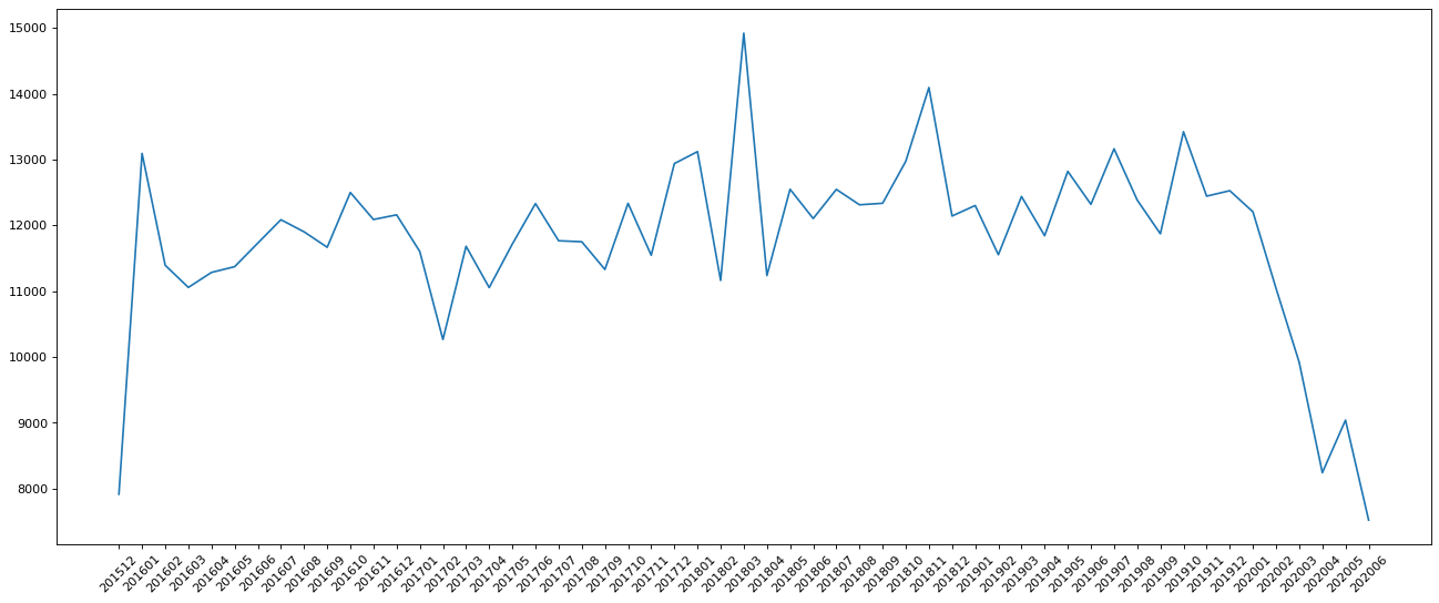
假设我们要统计这些数据中每个月的911紧急电话数量。
示例代码：

import pandas as pd
from matplotlib import pyplot as plt

d = pd.read_csv('911.csv')
# print(d.info())
# print(d.head())
print("=" * 6)

d['timeStamp'] = pd.to_datetime(d['timeStamp'])
d.set_index('timeStamp',inplace=True)
print("修改索引后")
print(d.head())

print("d.resample('M').count()  统计911数据中不同月份电话次数")
print(d.resample('M').count()[:5])

count_by_month = d.resample('M').count()['title']
_x = count_by_month.index
_y = count_by_month.values

_x = [i.strftime('%Y%m') for i in _x]

plt.figure(figsize=(20,8),dpi=80)
plt.plot(range(len(_x)),_y)
plt.xticks(range(len(_x)),_x,rotation=45)
plt.show()

运行结果：

======
修改索引后
                           lat        lng  \
timeStamp                                   
2015-12-10 17:10:52  40.297876 -75.581294   
2015-12-10 17:29:21  40.258061 -75.264680   
2015-12-10 14:39:21  40.121182 -75.351975   
2015-12-10 16:47:36  40.116153 -75.343513   
2015-12-10 16:56:52  40.251492 -75.603350   

                                                                  desc  \
timeStamp                                                                
2015-12-10 17:10:52  REINDEER CT & DEAD END;  NEW HANOVER; Station ...   
2015-12-10 17:29:21  BRIAR PATH & WHITEMARSH LN;  HATFIELD TOWNSHIP...   
2015-12-10 14:39:21  HAWS AVE; NORRISTOWN; 2015-12-10 @ 14:39:21-St...   
2015-12-10 16:47:36  AIRY ST & SWEDE ST;  NORRISTOWN; Station 308A;...   
2015-12-10 16:56:52  CHERRYWOOD CT & DEAD END;  LOWER POTTSGROVE; S...   

                         zip                    title                twp  \
timeStamp                                                                  
2015-12-10 17:10:52  19525.0   EMS: BACK PAINS/INJURY        NEW HANOVER   
2015-12-10 17:29:21  19446.0  EMS: DIABETIC EMERGENCY  HATFIELD TOWNSHIP   
2015-12-10 14:39:21  19401.0      Fire: GAS-ODOR/LEAK         NORRISTOWN   
2015-12-10 16:47:36  19401.0   EMS: CARDIAC EMERGENCY         NORRISTOWN   
2015-12-10 16:56:52      NaN           EMS: DIZZINESS   LOWER POTTSGROVE   

                                           addr  e  
timeStamp                                           
2015-12-10 17:10:52      REINDEER CT & DEAD END  1  
2015-12-10 17:29:21  BRIAR PATH & WHITEMARSH LN  1  
2015-12-10 14:39:21                    HAWS AVE  1  
2015-12-10 16:47:36          AIRY ST & SWEDE ST  1  
2015-12-10 16:56:52    CHERRYWOOD CT & DEAD END  1  
d.resample('M').count()  统计911数据中不同月份电话次数
              lat    lng   desc    zip  title    twp   addr      e
timeStamp                                                         
2015-12-31   7916   7916   7916   6902   7916   7911   7916   7916
2016-01-31  13096  13096  13096  11512  13096  13094  13096  13096
2016-02-29  11396  11396  11396   9926  11396  11395  11396  11396
2016-03-31  11059  11059  11059   9754  11059  11052  11059  11059
2016-04-30  11287  11287  11287   9897  11287  11284  11287  11287
<Figure size 1600x640 with 1 Axes>

链式索引

现象

问题

正常情况

创建DataFrame对象，示例代码：

import pandas as pd
import numpy as np

data = {"x": 2 ** np.arange(5),
        "y": 3 ** np.arange(5),
        "z": np.array([45, 98, 24, 11, 64])}

index = ["a", "b", "c", "d", "e"]

df = pd.DataFrame(data=data, index=index)

print(df)

运行结果：

    x   y   z
a   1   1  45
b   2   3  98
c   4   9  24
d   8  27  11
e  16  81  64

对x列进行赋值，这个也没有任何问题。示例代码：

1 2	df["x"] = 10 print(df)

运行结果：

    x   y   z
a  10   1  45
b  10   3  98
c  10   9  24
d  10  27  11
e  10  81  64

筛选出z列中所有小于50的记录，当然也是OK的。示例代码：

mask = df["z"] < 50
print(mask)
print(type(mask))

dfm = df[mask]
print(dfm)
print(type(dfm))

运行结果：

a     True
b    False
c     True
d     True
e    False
Name: z, dtype: bool
<class 'pandas.core.series.Series'>
    x   y   z
a  10   1  45
c  10   9  24
d  10  27  11
<class 'pandas.core.frame.DataFrame'>

解释说明：mask是一个有布尔值构成的Series对象，把mask作为df的索引，得到了按照筛选条件返回的记录，也是一个DataFrame对象。

有告警赋值成功

我们对上文的dfm的x列进行赋值。成功确实是成功了，但是有告警。

示例代码：

1 2	dfm['x'] = 100 print(dfm)

运行结果：

     x   y   z
a  100   1  45
c  100   9  24
d  100  27  11

SettingWithCopyWarning: 
A value is trying to be set on a copy of a slice from a DataFrame.
Try using .loc[row_indexer,col_indexer] = value instead

See the caveats in the documentation: https://pandas.pydata.org/pandas-docs/stable/user_guide/indexing.html#returning-a-view-versus-a-copy
  dfm['x'] = 100

我们还可以在这时候打印df看一下，没有被修改。
示例代码：

print(df)

运行结果：

    x   y   z
a   1   1  45
b   2   3  98
c   4   9  24
d   8  27  11
e  16  81  64

有告警且赋值失败

我们直接对符合mask条件的df的x列进行赋值。有告警且赋值失败。

示例代码：

1 2	df[mask]['x'] = 100 print(df)

运行结果：

    x   y   z
a  10   1  45
b  10   3  98
c  10   9  24
d  10  27  11
e  10  81  64

SettingWithCopyWarning: 
A value is trying to be set on a copy of a slice from a DataFrame.
Try using .loc[row_indexer,col_indexer] = value instead

See the caveats in the documentation: https://pandas.pydata.org/pandas-docs/stable/user_guide/indexing.html#returning-a-view-versus-a-copy
  df[mask]['x'] = 100

解决

copy()

dfm = dfm.copy()

对于问题一，在赋值之前，加上一行dfm = dfm.copy()，就不会有告警了。

示例代码：

1
2
3

dfm = dfm.copy()
dfm['x'] = 100
print(dfm)

运行结果：

     x   y   z
a  100   1  45
c  100   9  24
d  100  27  11

df = df.copy()

对于问题二，df = df.copy()，无效。

示例代码：

1
2
3

df = df.copy()
df[mask]['x'] = 100
print(df)

运行结果：

    x   y   z
a  10   1  45
b  10   3  98
c  10   9  24
d  10  27  11
e  10  81  64

SettingWithCopyWarning: 
A value is trying to be set on a copy of a slice from a DataFrame.
Try using .loc[row_indexer,col_indexer] = value instead

See the caveats in the documentation: https://pandas.pydata.org/pandas-docs/stable/user_guide/indexing.html#returning-a-view-versus-a-copy
  df[mask]['x'] = 100

loc[mask, “z”] = 100

该方法不用对问题一进行尝试，dfm是已经经过mask筛选之后的。
对于问题二，df.loc[mask, "x"] = 100，有效。

示例代码：

1 2	df.loc[mask, "x"] = 100 print(df)

运行结果：

     x   y   z
a  100   1  45
b   10   3  98
c  100   9  24
d  100  27  11
e   10  81  64

[‘x’][mask] = 100

对于问题二，df['x'][mask] = 100，有效。

示例代码：

1 2	df['x'][mask] = 100 print(df)

运行结果：

     x   y   z
a  100   1  45
b   10   3  98
c  100   9  24
d  100  27  11
e   10  81  64

loc[mask][“z”] = 0

如果我们把mask和"z"的前后顺序换一下，无效。

示例代码：

1
2
3

df.loc[mask]["z"] = 0

print(df)

运行结果：

    x   y   z
a  10   1  45
b  10   3  98
c  10   9  24
d  10  27  11
e  10  81  64

SettingWithCopyWarning: 
A value is trying to be set on a copy of a slice from a DataFrame.
Try using .loc[row_indexer,col_indexer] = value instead

See the caveats in the documentation: https://pandas.pydata.org/pandas-docs/stable/user_guide/indexing.html#returning-a-view-versus-a-copy
  df.loc[mask]["z"] = 0

weakref

关于什么情况下有weakref，什么情况下没有，确实还没总结出来。

有weakref的情况：

出现了链式索引，或者隐蔽的链式索引

没有weakref的有：

完全新建的
copy()之后的
loc[row_indexer,col_indexer]之后的

以下举几个例子。

完全新建的

完全新建的，没有weakref。

示例代码：

import pandas as pd
import numpy as np

data = {"x": 2 ** np.arange(5),
        "y": 3 ** np.arange(5),
        "z": np.array([45, 98, 24, 11, 64])}

index = ["a", "b", "c", "d", "e"]

df = pd.DataFrame(data=data, index=index)

print('df')
print(df)
print(df._is_view)
print(df._is_copy)

运行结果：

df
    x   y   z
a   1   1  45
b   2   3  98
c   4   9  24
d   8  27  11
e  16  81  64
False
None

注意，_is_copy的返回，没有weakref

有链式索引的

隐蔽的链式索引，示例代码：

dfa = df["a":"c"]
print(dfa)
print(dfa._is_view)
print(dfa._is_copy)

运行结果：

   x  y   z
a  1  1  45
b  2  3  98
c  4  9  24
True
<weakref at 0x7ff54ee92130; to 'DataFrame' at 0x7ff54a686850>

隐蔽的链式索引，示例代码：

dfb = df[:1]
print(dfb)
print(dfb._is_view)
print(dfb._is_copy)

运行结果：

   x  y   z
a  1  1  45
True
<weakref at 0x7f9999eb52c0; to 'DataFrame' at 0x7f9996d86850>

隐蔽的链式索引，示例代码：

dfc = df.loc[:'x']
print(dfc)
print(dfc._is_view)
print(dfc._is_copy)

运行结果：

    x   y   z
a   1   1  45
b   2   3  98
c   4   9  24
d   8  27  11
e  16  81  64
True
<weakref at 0x7fdb99eb5270; to 'DataFrame' at 0x7fdb95d86850>

未出现链式索引，示例代码：

dfd = df.iloc[2]
print(dfd)
print(dfd._is_view)
print(dfd._is_copy)

运行结果：

x     4
y     9
z    24
Name: c, dtype: int64
True
None

链式索引，示例代码：

dfm = df[df['x'] > 5]
print(dfm)
print(dfm._is_view)
print(dfm._is_copy)

运行结果：

    x   y   z
d   8  27  11
e  16  81  64
False
<weakref at 0x7fd8926b5180; to 'DataFrame' at 0x7fd88e286850>

copy()之后的

示例代码：

dfmc = dfm.copy()
print(dfmc)
print(dfmc._is_view)
print(dfmc._is_copy)

运行结果：

    x   y   z
d   8  27  11
e  16  81  64
False
None

loc[row_indexer,col_indexer]之后的

示例代码：

1	print(df.loc[df['x'] > 5, 'x']._is_copy)

运行结果：

None

上文现象的解释

如果有weakref，就会告警或报错，因为Pandas无法判断，你到底是要对那一个进行操作。

例如，a weakref from b，无法知道你是要操作a，还是b。

具体可以对每一个现象和解决进行验证，这里略。

解决方法

尽可能避免通过链式索引(隐蔽的链式索引)进行赋值。

有些资料的谬误

错误的例子

在有些资料中，会说DataFrame的copy()方法，如果deep=False是视图，deep=True是拷贝，默认deep=True。

还会进行如下的比较。

type一样，id不一样。

示例代码：

print(type(df))
print(type(view_of_df))
print(type(copy_of_df))

print(id(df))
print(id(view_of_df))
print(id(copy_of_df))

运行结果：

<class 'pandas.core.frame.DataFrame'>
<class 'pandas.core.frame.DataFrame'>
<class 'pandas.core.frame.DataFrame'>
140160986015824
140160985904800
140161055304288

转成Numpy数组，查看flags.owndata，都是False。

示例代码：

1
2
3

print(df.to_numpy().flags.owndata)
print(view_of_df.to_numpy().flags.owndata)
print(copy_of_df.to_numpy().flags.owndata)

运行结果：

1
2
3

False
False
False

转成Numpy数组，查看base。
df和view_of_df的base相同。

示例代码：

print(df.to_numpy().base)
print(view_of_df.to_numpy().base)
print(copy_of_df.to_numpy().base)

print(id(df.to_numpy().base))
print(id(view_of_df.to_numpy().base))
print(id(copy_of_df.to_numpy().base))

运行结果：

[[ 1  2  4  8 16]
 [ 1  3  9 27 81]
 [45 98 24 11 64]]
[[ 1  2  4  8 16]
 [ 1  3  9 27 81]
 [45 98 24 11 64]]
[[ 1  2  4  8 16]
 [ 1  3  9 27 81]
 [45 98 24 11 64]]

140456250522672
140456250522672
140456250521904

最后，会根据转成df后，共用了一个base，得出结论，deep=False是视图，deep=True是拷贝。

三者都是视图

无论deep=False或deep=True，都是拷贝，只是deep=True的时候是深拷贝。

我们可以试一下，如果deep=False是视图的话，那么修改原数据，视图也会被受影响，但实际没有。示例代码：

import pandas as pd
import numpy as np

data = {"x": 2 ** np.arange(5),
        "y": 3 ** np.arange(5),
        "z": np.array([45, 98, 24, 11, 64])}

index = ["a", "b", "c", "d", "e"]

df = pd.DataFrame(data=data, index=index)
view_of_df = df.copy(deep=False)
copy_of_df = df.copy()

df[["z"]] = 0
print(df)
print(view_of_df)
print(copy_of_df)

运行结果：

    x   y  z
a   1   1  0
b   2   3  0
c   4   9  0
d   8  27  0
e  16  81  0
    x   y   z
a   1   1  45
b   2   3  98
c   4   9  24
d   8  27  11
e  16  81  64
    x   y   z
a   1   1  45
b   2   3  98
c   4   9  24
d   8  27  11
e  16  81  64

其实，三者都不是视图。示例代码：

1
2
3

print(df._is_view)
print(view_of_df._is_view)
print(copy_of_df._is_view)

运行结果：

1
2
3

False
False
False

计算方法

cumprod

使用方法

Pandas中的cumprod()函数用于计算给定序列的累积乘积。它返回一个与原始序列长度相同的新序列，其中每个元素都是原始序列中该位置及之前所有元素的乘积。
具体来说，cumprod()函数的作用是将序列中的每个元素依次相乘，并返回一个新序列，其中第i个元素是原始序列中前i个元素的乘积。

cumprod()函数的语法如下：

1	pandas.DataFrame.cumprod(axis=None, skipna=True, args, *kwargs)

axis参数用于指定计算累积乘积的轴
skipna参数用于指定是否跳过缺失值。
- 如果skipna=True，则在计算累积乘积时会将跳过缺失值。
- 如果skipna=False，则在计算累积乘积时不会跳过，连乘计算后是NaN。
- 默认skipna=True。

例子

示例代码：

# 创建一个序列
s = pd.Series([1, 2, 3, 4, 5])

# 计算序列的累积乘积
cumprod = s.cumprod()

# 输出结果
print(cumprod)

运行结果：

0      1
1      2
2      6
3     24
4    120
dtype: int64

skipna=True，示例代码：

# 创建一个序列
s = pd.Series([1, 2, None, 4, 5])

# 计算序列的累积乘积
cumprod = s.cumprod(skipna=True)

# 输出结果
print(cumprod)

运行结果：

0     1.0
1     2.0
2     NaN
3     8.0
4    40.0
dtype: float64

默认skipna=True，示例代码：

# 创建一个序列
s = pd.Series([1, 2, None, 4, 5])

# 计算序列的累积乘积
cumprod = s.cumprod()

# 输出结果
print(cumprod)

运行结果：

0     1.0
1     2.0
2     NaN
3     8.0
4    40.0
dtype: float64

skipna=False，不跳过。示例代码：

# 创建一个序列
s = pd.Series([1, 2, None, 4, 5])

# 计算序列的累积乘积
cumprod = s.cumprod(skipna=False)

# 输出结果
print(cumprod)

运行结果：

0    1.0
1    2.0
2    NaN
3    NaN
4    NaN
dtype: float64

还有一个cumsum()，作用相同。

shift

使用方法

shift()，将DataFrame或Series中的数据按给定数量的轴移动，在处理时间序列数据时非常有用。

1	DataFrame.shift(periods=1, freq=None, axis=0, fill_value=_NoDefault.no_default)

常用参数：

periods：移动的步数，默认1
axis：
- 0，index
- 1，columns
- 默认0

例子

默认是对所有的行或列进行平移，可以通过如下的方式，指定某一列

1	df['Col3Shift'] = df['Col3'].shift(periods=1)

示例代码：

import pandas as pd

df = pd.DataFrame({"Col1": [10, 20, 15, 30, 45],
                   "Col2": [13, 23, 18, 33, 48],
                   "Col3": [17, 27, 22, 37, 52]},
                  index=pd.date_range("2020-01-01", "2020-01-05"))

print(df)

print(df.shift(periods=3))

print(df.shift(periods=1, axis="columns"))

df['Col3Shift'] = df['Col3'].shift(periods=1)

print(df)

运行结果：

            Col1  Col2  Col3
2020-01-01    10    13    17
2020-01-02    20    23    27
2020-01-03    15    18    22
2020-01-04    30    33    37
2020-01-05    45    48    52
            Col1  Col2  Col3
2020-01-01   NaN   NaN   NaN
2020-01-02   NaN   NaN   NaN
2020-01-03   NaN   NaN   NaN
2020-01-04  10.0  13.0  17.0
2020-01-05  20.0  23.0  27.0
            Col1  Col2  Col3
2020-01-01   NaN    10    13
2020-01-02   NaN    20    23
2020-01-03   NaN    15    18
2020-01-04   NaN    30    33
2020-01-05   NaN    45    48
            Col1  Col2  Col3  Col3Shift
2020-01-01    10    13    17        NaN
2020-01-02    20    23    27       17.0
2020-01-03    15    18    22       27.0
2020-01-04    30    33    37       22.0
2020-01-05    45    48    52       37.0

计算回报率，示例代码：

import pandas as pd
df = pd.DataFrame({'Date': [1, 2, 3, 4],'Price': [13.02, 13.10, 13.35, 13.91]})

print(df)

df['shifted'] = df['Price'].shift(periods=1)
print(df)

df['return'] = (df['Price'] / df['shifted']) - 1
print(df)

运行结果：

   Date  Price
0     1  13.02
1     2  13.10
2     3  13.35
3     4  13.91
   Date  Price  shifted
0     1  13.02      NaN
1     2  13.10    13.02
2     3  13.35    13.10
3     4  13.91    13.35
   Date  Price  shifted    return
0     1  13.02      NaN       NaN
1     2  13.10    13.02  0.006144
2     3  13.35    13.10  0.019084
3     4  13.91    13.35  0.041948

比较股票价格与移动平均价格之间的百分比变化，示例代码：

import pandas as pd
df = pd.DataFrame({'Price': [10.4, 13.2, 12.9, 10.2, 11.5]})
print('df')
print(df)

rolling_mean = df.rolling(window=2).mean()
print('rolling_mean')
print(rolling_mean)

shifted = df.shift(periods=1)
print('shifted')
print(shifted)

percent_change = (df - shifted) / shifted
print('percent_change')
print(percent_change)

percent_change_from_mean = (df - rolling_mean) / rolling_mean
print('percent_change_from_mean')
print(percent_change_from_mean)

运行结果：

df
   Price
0   10.4
1   13.2
2   12.9
3   10.2
4   11.5
rolling_mean
   Price
0    NaN
1  11.80
2  13.05
3  11.55
4  10.85
shifted
   Price
0    NaN
1   10.4
2   13.2
3   12.9
4   10.2
percent_change
      Price
0       NaN
1  0.269231
2 -0.022727
3 -0.209302
4  0.127451
percent_change_from_mean
      Price
0       NaN
1  0.118644
2 -0.011494
3 -0.116883
4  0.059908

计算日股价变化的标准差，示例代码：

import pandas as pd
df = pd.DataFrame({'Price': [10.4, 13.2, 12.9, 10.2, 11.5]})
print('df')
print(df)

shifted = df.shift(periods=1)
print('shifted')
print(shifted)

daily_return = df / shifted - 1
print('daily_return')
print(daily_return)

rolling_std = daily_return.rolling(window=2).std()
print('rolling_std')
print(rolling_std)

运行结果：

df
   Price
0   10.4
1   13.2
2   12.9
3   10.2
4   11.5
shifted
   Price
0    NaN
1   10.4
2   13.2
3   12.9
4   10.2
daily_return
      Price
0       NaN
1  0.269231
2 -0.022727
3 -0.209302
4  0.127451
rolling_std
      Price
0       NaN
1       NaN
2  0.206446
3  0.131928
4  0.238121

diff

使用方法

diff，用于计算每个元素与其相邻元素之间的差异。

1	DataFrame.diff(periods=1, axis=0)

常用参数：

periods，表示向前计算的位置。默认为1，可以是正整数或负整数。
axis
- 0，index
- 1，columns
- 默认，0

例子

示例代码：

import pandas as pd

df = pd.DataFrame({'a': [1, 2, 3, 4, 5, 6],
                   'b': [1, 1, 2, 3, 5, 8],
                   'c': [1, 4, 9, 16, 25, 36]})
print(df)

print(df.diff())

print(df.diff(axis=1))

print(df.diff(periods=3))

print(df.diff(periods=-1))

运行结果：

   a  b   c
0  1  1   1
1  2  1   4
2  3  2   9
3  4  3  16
4  5  5  25
5  6  8  36
     a    b     c
0  NaN  NaN   NaN
1  1.0  0.0   3.0
2  1.0  1.0   5.0
3  1.0  1.0   7.0
4  1.0  2.0   9.0
5  1.0  3.0  11.0
    a  b   c
0 NaN  0   0
1 NaN -1   3
2 NaN -1   7
3 NaN -1  13
4 NaN  0  20
5 NaN  2  28
     a    b     c
0  NaN  NaN   NaN
1  NaN  NaN   NaN
2  NaN  NaN   NaN
3  3.0  2.0  15.0
4  3.0  4.0  21.0
5  3.0  6.0  27.0
     a    b     c
0 -1.0  0.0  -3.0
1 -1.0 -1.0  -5.0
2 -1.0 -1.0  -7.0
3 -1.0 -2.0  -9.0
4 -1.0 -3.0 -11.0
5  NaN  NaN   NaN

计算股票价格变化率，示例代码：

import pandas as pd

df = pd.DataFrame({'Price': [12.04, 10.91, 10.71, 9.71, 10.01, 10.05]})

print('df')
print(df)

diff = df['Price'].diff()
print('diff')
print(diff)

shift = df['Price'].shift()
print('shift')
print(shift)

change = diff / shift
print('change')
print(change)

运行结果：

df
   Price
0  12.04
1  10.91
2  10.71
3   9.71
4  10.01
5  10.05
diff
0     NaN
1   -1.13
2   -0.20
3   -1.00
4    0.30
5    0.04
Name: Price, dtype: float64
shift
0      NaN
1    12.04
2    10.91
3    10.71
4     9.71
5    10.01
Name: Price, dtype: float64
change
0         NaN
1   -0.093854
2   -0.018332
3   -0.093371
4    0.030896
5    0.003996
Name: Price, dtype: float64

计算统计差异，示例代码：

import pandas as pd
df = pd.DataFrame({'A': [10, 20, 15, 30, 45], 'B': [10, 15, 5, 25, 40]})
print(df)

diff = df.diff(axis=1)
print(diff)

运行结果：

periods参数设置为3时，计算每个元素与其前三个元素之间的差异。示例代码：

import pandas as pd
s = pd.Series([10, 15, 13, 12, 11, 14, 13])
print(s)

change = s.diff(periods=3)
print(change)

运行结果：

0    10
1    15
2    13
3    12
4    11
5    14
6    13
dtype: int64
0    NaN
1    NaN
2    NaN
3    2.0
4   -4.0
5    1.0
6    1.0
dtype: float64

pct_change

使用方法

pct_change，用于计算序列数据中每个元素与其前一个元素的变化率。

举例来说：

diff
df[‘column’].diff(-1)，计算column列这一行减去上一行数据之差。
pct_change
df[‘column’].pct_change(-1)，计算column列这一行减去上一行数据之差再除以上一行，即每日涨跌幅。

1	DataFrame.pct_change(periods=1, fill_method='pad', limit=None, freq=None, **kwargs)

常用参数：

periods: 要计算差异的步数。默认值为1，这意味着要计算每个元素与其前一个元素之间的差异。
fill_method：'backfill'、'bfill'、'pad'、'ffill'、None，默认'pad'。

例子

示例代码：

import pandas as pd
s = pd.Series([90, 91, 85])
print(s)

print(s.pct_change())

运行结果：

0    90
1    91
2    85
dtype: int64
0         NaN
1    0.011111
2   -0.065934
dtype: float64

计算季度变化，示例代码：

import pandas as pd

data = {'Quarter': [1, 1, 1, 2, 2, 2, 3, 3, 3, 4, 4, 4],
        'Year': [2018, 2019, 2020, 2018, 2019, 2020, 2018, 2019, 2020, 2018, 2019, 2020],
        'Price': [100, 101, 98, 103, 105, 98, 110, 111, 115, 120, 124, 125]}
df = pd.DataFrame(data)
print(df)

df.set_index(['Year', 'Quarter'], inplace=True)
change = df['Price'].pct_change(periods=1)
print(change)

运行结果：

    Quarter  Year  Price
0         1  2018    100
1         1  2019    101
2         1  2020     98
3         2  2018    103
4         2  2019    105
5         2  2020     98
6         3  2018    110
7         3  2019    111
8         3  2020    115
9         4  2018    120
10        4  2019    124
11        4  2020    125
Year  Quarter
2018  1               NaN
2019  1          0.010000
2020  1         -0.029703
2018  2          0.051020
2019  2          0.019417
2020  2         -0.066667
2018  3          0.122449
2019  3          0.009091
2020  3          0.036036
2018  4          0.043478
2019  4          0.033333
2020  4          0.008065
Name: Price, dtype: float64

periods参数设置为3时，计算每个元素与其前第三个元素之间的差异。示例代码：

import pandas as pd
s = pd.Series([10, 15, 13, 12, 11, 14, 13])
print(s)

change = s.pct_change(periods=3)
print(change)

运行结果：

0    10
1    15
2    13
3    12
4    11
5    14
6    13
dtype: int64
0         NaN
1         NaN
2         NaN
3    0.200000
4   -0.266667
5    0.076923
6    0.083333
dtype: float64

rolling

使用方法

rolling()，主要用于计算滚动窗口自相关，窗口函数(如移动平均值和移动标准差)等统计指标。

1	DataFrame.rolling(window, min_periods=None, center=False, win_type=None, on=None, axis=0, closed=None, step=None, method='single')

常用参数：

window，表示滚动计算的窗口大小。默认为1，表示每个元素都被单独计算处理。该参数可以是正整数，用于指定计算差异的时间跨度。
min_periods，最少所需的非NA值来计算每个元素的值。默认值为None，但在某些函数中具有其他默认值(如var()为窗口大小)。

例子

计算股票价格移动平均线，示例代码：

import pandas as pd

df = pd.DataFrame({'Price': [12.04, 10.91, 10.71, 9.71, 10.01, 10.05]})
print(df)

rolling_mean = df['Price'].rolling(window=2).mean()
print(rolling_mean)

运行结果：

   Price
0  12.04
1  10.91
2  10.71
3   9.71
4  10.01
5  10.05
0       NaN
1    11.475
2    10.810
3    10.210
4     9.860
5    10.030
Name: Price, dtype: float64

计算MACD，示例代码：

import pandas as pd

df = pd.DataFrame({'Price': [12.04, 10.91, 10.71, 9.71, 10.01, 10.05]})
print(df)

short_rolling = df.rolling(window=2).mean()
long_rolling = df.rolling(window=4).mean()
macd = short_rolling - long_rolling
print(macd)

运行结果：

   Price
0  12.04
1  10.91
2  10.71
3   9.71
4  10.01
5  10.05
    Price
0     NaN
1     NaN
2     NaN
3 -0.6325
4 -0.4750
5 -0.0900

计算移动股票成交量的标准差，示例代码：

import pandas as pd

df = pd.DataFrame({'Volume': [175000, 250000, 310000, 210000, 180000]})
print(df)

rolling_std = df['Volume'].rolling(window=2).std()
print(rolling_std)

运行结果：

   Volume
0  175000
1  250000
2  310000
3  210000
4  180000
0             NaN
1    53033.008589
2    42426.406871
3    70710.678119
4    21213.203436
Name: Volume, dtype: float64

transform

使用方法

transform()，主要用于基于组计算或函数向数据集的每个元素应用函数并返回与原始DataFrame或Series对象类型相同的数据集。

1	DataFrame.transform(func, axis=0, args, *kwargs)

transform()函数有一个主要参数，func，表示要应用于每个元素的函数。也可以使用lambda函数或numpy函数作为此参数。

例子

transform()，计算组内元素的平均值。示例代码：

import pandas as pd

df = pd.DataFrame({'A': ['a', 'b', 'a', 'c', 'b', 'a'], 'B': [1, 2, 3, 4, 5, 6]})
print(df)

transformed = df.groupby('A')['B'].transform(lambda x: x.mean())
print(transformed)

运行结果：

   A  B
0  a  1
1  b  2
2  a  3
3  c  4
4  b  5
5  a  6
0    3.333333
1    3.500000
2    3.333333
3    4.000000
4    3.500000
5    3.333333
Name: B, dtype: float64

标准化股票价格，示例代码：

import pandas as pd
from scipy import stats

df = pd.DataFrame({'Price': [20.5, 23.4, 19.7, 22.0, 18.4], 'Volume': [20000, 31000, 24000, 18000, 28000]})
print(df)

df['Price_Zscore'] = df['Price'].transform(lambda x: (x - x.mean()) / x.std())
df['Price_Zscore_stats_1'] = stats.zscore(df['Price'],ddof=1)
df['Price_Zscore_stats_0'] = stats.zscore(df['Price'],ddof=0)

print(df)

运行结果：

   Price  Volume
0   20.5   20000
1   23.4   31000
2   19.7   24000
3   22.0   18000
4   18.4   28000
   Price  Volume  Price_Zscore  Price_Zscore_stats_1  Price_Zscore_stats_0
0   20.5   20000     -0.153594             -0.153594             -0.171723
1   23.4   31000      1.331147              1.331147              1.488268
2   19.7   24000     -0.563178             -0.563178             -0.629652
3   22.0   18000      0.614376              0.614376              0.686893
4   18.4   28000     -1.228751             -1.228751             -1.373786

缺失值处理，示例代码：

import pandas as pd
import numpy as np

df = pd.DataFrame({'A': ['a', 'a', 'b', 'b', 'c', 'c'], 'B': [1, np.nan, np.nan, 4, 5, 6]})
print(df)

df['B_fill_Nan'] = df.groupby('A')['B'].transform(lambda x: x.fillna(x.mean()))
print(df)

运行结果：

   A    B
0  a  1.0
1  a  NaN
2  b  NaN
3  b  4.0
4  c  5.0
5  c  6.0
   A    B  B_fill_Nan
0  a  1.0         1.0
1  a  NaN         1.0
2  b  NaN         4.0
3  b  4.0         4.0
4  c  5.0         5.0
5  c  6.0         6.0

计算股票交易量的排名，示例代码：

import pandas as pd

df = pd.DataFrame({'Price': [13.2, 14.3, 13.6, 14.1, 13.8], 'Volume': [20000, 31000, 24000, 18000, 28000]})
print(df)

df['Rank'] = df['Volume'].transform(lambda x: x.rank(method='dense', ascending=False))
print(df)

运行结果：

   Price  Volume
0   13.2   20000
1   14.3   31000
2   13.6   24000
3   14.1   18000
4   13.8   28000
   Price  Volume  Rank
0   13.2   20000   4.0
1   14.3   31000   1.0
2   13.6   24000   3.0
3   14.1   18000   5.0
4   13.8   28000   2.0

rank

使用方法

rank()给DataFrame或Series中的值排名，并且可以指定排名规则，比如升序排列或降序排列。

1	DataFrame.rank(axis=0, method='average', numeric_only=False, na_option='keep', ascending=True, pct=False)

常用参数：

axis
- 0，index
- 1，columns
- 默认，0
method：指定排名规则，可选的参数有average、min、max、first，分别表示对于排名相同的数值，用平均值、最小值、最大值、首个出现的值计算排名，默认为average。
ascending：指定是否升序排列，默认为True表示升序排列。
pct：当为True时，结果为分位数，即在原始数据中排名超过多少百分比。
na_option：指定处理缺失值，可选的参数有keep、top、bottom，分别表示保留缺失值、把缺失值放在最前面或最后面，默认为keep。

例子

示例代码：

import pandas as pd
import numpy as np

# 生成一个DataFrame
df = pd.DataFrame({'A': [1, 2, 3, 4], 
                   'B': [3, np.nan, 5, 3], 
                   'C': [2, 6, 5, 1]}, index=['a', 'b', 'c', 'd'])
print('df')
print(df)

# 对列B按升序排名
df['B_rank'] = df['B'].rank(ascending=True)
print('对列B按升序排名')
print(df)

# 对列B按降序排名，并指定排名相同的项用最大值计算排名
df['B_rank'] = df['B'].rank(ascending=False, method='max')
print('对列B按降序排名，并指定排名相同的项用最大值计算排名')
print(df)

运行结果：

df
   A    B  C
a  1  3.0  2
b  2  NaN  6
c  3  5.0  5
d  4  3.0  1
对列B按升序排名
   A    B  C  B_rank
a  1  3.0  2     1.5
b  2  NaN  6     NaN
c  3  5.0  5     3.0
d  4  3.0  1     1.5
对列B按降序排名，并指定排名相同的项用最大值计算排名
   A    B  C  B_rank
a  1  3.0  2     3.0
b  2  NaN  6     NaN
c  3  5.0  5     1.0
d  4  3.0  1     3.0

假设存在一组股票数据，按照收盘价计算排名，并计算前五名的股票的收盘价均值和涨跌幅。示例代码：

import pandas as pd

df = pd.DataFrame({'code': ['AAPL', 'GOOG', 'MSFT', 'AMZN', 'FB', 'TSLA'],
                   'close': [119.21, 1845.06, 202.68, 3099.96, 280.36, 555.77]})
print('df')
print(df)

df['rank'] = df['close'].rank(ascending=False)
print('df[\'rank\']')
print(df)

top5_mean_close = df.sort_values(by='rank').iloc[:5]['close'].mean()
print('top5_mean_close:', top5_mean_close)

运行结果：

df
   code    close
0  AAPL   119.21
1  GOOG  1845.06
2  MSFT   202.68
3  AMZN  3099.96
4    FB   280.36
5  TSLA   555.77
df['rank']
   code    close  rank
0  AAPL   119.21   6.0
1  GOOG  1845.06   2.0
2  MSFT   202.68   5.0
3  AMZN  3099.96   1.0
4    FB   280.36   4.0
5  TSLA   555.77   3.0
top5_mean_close: 1196.766

sample

使用方法

sample()，用于从数据集中随机抽取样本。

1	DataFrame.sample(n=None, frac=None, replace=False, weights=None, random_state=None, axis=None, ignore_index=False)

n，int，可选。

指定要抽取的样本数量，不能与frac一起使用。

示例代码：

import pandas as pd
import numpy as np

s = pd.Series(np.random.randint(0, 10, size=10))

print(s)

s = s.sample(n=3)

print(s)

运行结果：

0    8
1    9
2    4
3    9
4    8
5    3
6    8
7    6
8    4
9    1
dtype: int64
2    4
6    8
3    9
dtype: int64

frac，float，可选。

指定要抽取的样本比例，取值范围为 $[0,1]$ ，不能与n一起使用。

示例代码：

import pandas as pd
import numpy as np

s = pd.Series(np.random.randint(0, 10, size=10))

print(s)

s = s.sample(frac=0.4)

print(s)

运行结果：

1    7
2    8
3    4
4    5
5    7
6    9
7    6
8    2
9    0
dtype: int64
4    5
9    0
3    4
6    9
dtype: int64

frac，还有一个作用。当值为1时，可以对数据进行乱序。

示例代码：

import pandas as pd
import numpy as np

s = pd.Series(np.random.randint(0, 10, size=10))

print(s)

s = s.sample(frac=1)

print(s)

运行结果：

0    6
1    4
2    2
3    0
4    4
5    8
6    4
7    8
8    6
9    0
dtype: int64
4    4
0    6
9    0
7    8
2    2
6    4
5    8
8    6
1    4
3    0
dtype: int64

replace，bool，默认为False。

是否进行抽样重复，即是否"有放回的抽样"。

如果为True，则样本中可能会重复出现。
如果为False，不进行抽样重复。

示例代码：

import pandas as pd
import numpy as np

s = pd.Series(np.random.randint(0, 10, size=4))

print(s)

s = s.sample(n=3, replace=True)

print(s)

运行结果：

0    3
1    9
2    4
3    9
dtype: int64
0    3
0    3
0    3
dtype: int64

weights，指定每个元素被抽取的权重。

例如，从一个包含5个元素的Series中随机抽取3个元素。5个元素的权重分别是1、2、3、4、5。

示例代码：

import pandas as pd
import numpy as np

s = pd.Series(np.random.randint(0, 10, size=5))

print(s)

weights = [1, 2, 3, 4, 5]
s = s.sample(n=3, replace=True)

print(s)

运行结果：

0    4
1    0
2    7
3    1
4    9
dtype: int64
2    7
1    0
2    7
dtype: int64

例子

从一个包含股票交易数据的DataFrame中，随机抽取10%的交易记录，并计算抽样结果的交易量总和。示例代码：

import pandas as pd

trades = pd.DataFrame({'Stock': ['AAPL', 'AAPL', 'GOOG', 'GOOG', 'MSFT', 'MSFT', 'AAPL', 'GOOG'],
                       'Date': ['2021-01-01', '2021-01-01', '2021-01-01', '2021-01-01',
                                '2021-01-01', '2021-01-01', '2021-01-01', '2021-01-01'],
                       'Volume': [100, 200, 150, 50, 300, 100, 250, 180]})

sampled_trades = trades.sample(frac=0.1)
print(sampled_trades['Volume'].sum())

运行结果：

Panel

什么是Panel

Panel，面板，3维数据的存储结构，相当于一个存储DataFrame的字典，3个轴(axis)分别代表意义如下:

axis0，items，item对应一个内部的数据帧(DataFrame)。
axis1，major_axis，每个数据帧(DataFrame)的索引行。
axis2，minor_axis，每个数据帧(DataFrame)的索引列。

构造方法

pandas.Panel()，可以使用以下构造函数创建Panel。

1	pandas.Panel(data, items, major_axis, minor_axis, dtype, copy)

参数说明如下：

data，支持多种数据类型，如：ndarray、series，map，lists，dict，constant和其他数据帧(DataFrame)。
items，axis=0
major_axis，axis=1
minor_axis，axis=2
dtype，每列的数据类型
copy，是否复制数据，默认为false

创建Panel

创建一个空Panel

示例代码：

1
2
3

import pandas as pd
p = pd.Panel()
print (p)

运行结果：

<class 'pandas.core.panel.Panel'>
Dimensions: 0 (items) x 0 (major_axis) x 0 (minor_axis)
Items axis: None
Major_axis axis: None
Minor_axis axis: None

从3D-ndarray创建Panel

示例代码：

import pandas as pd
import numpy as np

data = np.random.rand(2, 4, 5)
p = pd.Panel(data)
print (p)

运行结果：

<class 'pandas.core.panel.Panel'>
Dimensions: 2 (items) x 4 (major_axis) x 5 (minor_axis)
Items axis: 0 to 1
Major_axis axis: 0 to 3
Minor_axis axis: 0 to 4

从DataFrame字典创建Panel

示例代码：

import pandas as pd
import numpy as np

data = {'Item1' : pd.DataFrame(np.random.randn(4, 3)), 
        'Item2' : pd.DataFrame(np.random.randn(4, 2))}
p = pd.Panel(data)
print (p)

运行结果：

<class 'pandas.core.panel.Panel'>
Dimensions: 2 (items) x 4 (major_axis) x 3 (minor_axis)
Items axis: Item1 to Item2
Major_axis axis: 0 to 3
Minor_axis axis: 0 to 2

读取数据

要从Panel中读取数据，可以使用以下方式：

Items
Major_axis
Minor_axis

使用Items

示例代码：

import pandas as pd
import numpy as np
data = {'Item1' : pd.DataFrame(np.random.randn(4, 3)), 
        'Item2' : pd.DataFrame(np.random.randn(4, 2))}
p = pd.Panel(data)
print (p['Item1'])

运行结果：

          0         1         2
0 -1.556207  0.193622 -0.316143
1 -0.538768 -0.753225  0.484204
2 -0.351821 -1.318368 -0.051768
3  1.275915 -0.033563 -0.199769

使用major_axis

示例代码：

import pandas as pd
import numpy as np
data = {'Item1' : pd.DataFrame(np.random.randn(4, 3)), 
        'Item2' : pd.DataFrame(np.random.randn(4, 2))}
p = pd.Panel(data)
print (p.major_xs(1))

运行结果：

      Item1     Item2
0  0.952543 -0.449554
1  0.671768 -0.851572
2 -1.298728       NaN

使用minor_axis

示例代码：

import pandas as pd
import numpy as np
data = {'Item1' : pd.DataFrame(np.random.randn(4, 3)), 
        'Item2' : pd.DataFrame(np.random.randn(4, 2))}
p = pd.Panel(data)
print (p.minor_xs(1))

运行结果：

      Item1     Item2
0  0.949440 -1.430323
1 -0.020717  0.474649
2 -2.015678 -0.227942
3 -1.012188 -1.318397

swapaxes

互换坐标轴。

示例代码：

import pandas as pd
import numpy as np
data = {'Item1' : pd.DataFrame(np.random.randn(4, 3)), 
        'Item2' : pd.DataFrame(np.random.randn(4, 2))}
p = pd.Panel(data)

print(p['Item1'])

print(p.minor_xs(1))

p = p.swapaxes("minor_axis", "items")

print(p[1])

运行结果：

          0         1         2
0  0.162309 -0.178309 -1.448816
1  0.236601  0.077832 -1.087040
2  0.611931  0.376039 -1.646674
3  0.236116 -1.872312 -0.233127
      Item1     Item2
0 -0.178309  0.553583
1  0.077832 -0.406340
2  0.376039  0.973701
3 -1.872312  2.434925
      Item1     Item2
0 -0.178309  0.553583
1  0.077832 -0.406340
2  0.376039  0.973701
3 -1.872312  2.434925

astype

astype(int)

astype(int)，只取整数部分，向下取整。

示例代码：

import pandas as pd
import numpy as np

df = pd.DataFrame(np.random.rand(3,4), columns=list("ABCD"))
print(df)
df[list("ABCD")] = df[list("ABCD")].astype(int)
print(df)

运行结果：

          A         B         C         D
0  0.413756  0.414248  0.420190  0.494105
1  0.285176  0.577459  0.308047  0.631833
2  0.722435  0.001823  0.196517  0.561772
   A  B  C  D
0  0  0  0  0
1  0  0  0  0
2  0  0  0  0

astype(float)

现象

这个现象，不一定在每一个版本的Python或者Pandas中都会复现。

注意，其中的price，有多种类型的数据，示例代码：

import pandas as pd

extracted_data = pd.DataFrame({
    'Brand': ['Gucci', 'Nike', 'Adidas', 'Hermes', 'Zara'],
    'year_of_manufacture': [2010, 1999, '2012', 2011, '2008'],
    'price': ['4034.203', 5000.00, '7450.17567', 3023.004, '4901.32345']
})

extracted_data['price'] = extracted_data['price'].round(2)

print(extracted_data)

运行结果：

TypeError                                 Traceback (most recent call last)
Cell In[6], line 9
      1 import pandas as pd
      3 extracted_data = pd.DataFrame({
      4     'Brand': ['Gucci', 'Nike', 'Adidas', 'Hermes', 'Zara'],
      5     'year_of_manufacture': [2010, 1999, '2012', 2011, '2008'],
      6     'price': ['4034.203', 5000.00, '7450.17567', 3023.004, '4901.32345']
      7 })
----> 9 extracted_data['price'] = extracted_data['price'].round(2)
     11 print(extracted_data)

File ~/anaconda3/lib/python3.10/site-packages/pandas/core/series.py:2602, in Series.round(self, decimals, *args, **kwargs)
   2570 """
   2571 Round each value in a Series to the given number of decimals.
   2572 
   (...)
   2599 dtype: float64
   2600 """
   2601 nv.validate_round(args, kwargs)
-> 2602 result = self._values.round(decimals)
   2603 result = self._constructor(result, index=self.index).__finalize__(
   2604     self, method="round"
   2605 )
   2607 return result

TypeError: can't multiply sequence by non-int of type 'float'

解决

用astype进行类型转换，转成float类型。示例代码：

import pandas as pd

extracted_data = pd.DataFrame({
    'Brand': ['Gucci', 'Nike', 'Adidas', 'Hermes', 'Zara'],
    'year_of_manufacture': [2010, 1999, '2012', 2011, '2008'],
    'price': ['4034.203', 5000.00, '7450.17567', 3023.004, '4901.32345']
})

cast_to_type = {
    'year_of_manufacture': int,
    'price': float
    }
extracted_data = extracted_data.astype(cast_to_type)

extracted_data['price'] = extracted_data['price'].round(2)

print(extracted_data)

运行结果：

    Brand  year_of_manufacture    price
0   Gucci                 2010  4034.20
1    Nike                 1999  5000.00
2  Adidas                 2012  7450.18
3  Hermes                 2011  3023.00
4    Zara                 2008  4901.32

set_option

显示所有列：pd.set_option('display.max_columns', None)
设置一行的宽度：pd.set_option('display.width', 5000)
显示所有行：pd.set_option('display.max_rows', None)
设置value的显示长度为100，默认为50：pd.set_option('max_colwidth',100)

参考资料：

https://book.itheima.net/course/221/1270308811000782849/1271373631313682433

https://book.itheima.net/course/221/1270308811000782849/1271373631317876737

https://book.itheima.net/course/221/1270308811000782849/1271373631326265345

https://pandas.pydata.org/docs/reference/api/pandas.DataFrame.shift.html

https://pandas.pydata.org/docs/reference/api/pandas.DataFrame.diff.html

https://pandas.pydata.org/docs/reference/api/pandas.DataFrame.pct_change.html

https://blog.csdn.net/The_Time_Runner/article/details/104559986

https://pandas.pydata.org/docs/reference/api/pandas.DataFrame.rolling.html

https://pandas.pydata.org/docs/reference/api/pandas.DataFrame.transform.html

https://pandas.pydata.org/docs/reference/api/pandas.DataFrame.rank.html

https://geek-docs.com/pandas/pandas-tutorials/python_pandas.html

https://dev.to/theolakusibe/solving-attributeerror-float-object-has-no-attribute-rint-4la

文章作者: Kaka Wan Yifan

文章链接: https://kakawanyifan.com/10303

评论区

概述

Series

Series的创建

通过list创建

通过字典创建

Series的索引

索引的操作

索引的属性

Series的值

DataFrame

DataFrame的创建

通过list创建

通过字典创建

DataFrame的属性

DataFrame的索引

简单的取行和取列操作

loc和iloc

布尔索引

reset_index

索引的其他操作

DataFrame的合并

join

merge

concat

DataFrame的读写

读写CSV

read_csv()

to_csv

读写Excel

read_excel

to_excel

读写数据库

SQLAlchemy

read_sql

to_sql

常用统计函数

分组聚合

根据单一属性进行分组聚合

根据多个属性进行分组聚合

时间序列

Pandas中的时间

to_datetime

支持的时间格式

生成时间范围

重采样

链式索引

现象

问题

正常情况

有告警赋值成功

有告警且赋值失败

解决

copy()

dfm = dfm.copy()

df = df.copy()

loc[mask, “z”] = 100

[‘x’][mask] = 100

loc[mask][“z”] = 0

weakref

完全新建的

有链式索引的

copy()之后的

loc[row_indexer,col_indexer]之后的

上文现象的解释

解决方法

有些资料的谬误

错误的例子

三者都是视图

计算方法

cumprod

使用方法

例子

shift

使用方法

例子

diff

使用方法

例子

pct_change

使用方法

通过`list`创建

通过`list`创建